Quantcast
Channel: Search Results for “maps”– R-bloggers
Viewing all 589 articles
Browse latest View live

Towards (Yet) Another R Colour Palette Generator. Step One: Quentin Tarantino.

$
0
0

(This article was first published on Blend it like a Bayesian!, and kindly contributed to R-bloggers)


Why?

I love colours, I love using colours even more. Unfortunately, I have to admit that I don't understand colours well enough to use them properly. It is the same frustration that I had about one year ago when I first realised that I couldn't plot anything better than the defaults in Excel and Matlab! It was for that very reason, I decided to find a solution and eventually learned R. Still learning it today.

What's wrong with my previous attempts to use colours? Let's look at CrimeMap. The colour choices, when I first created the heatmaps, were entirely based on personal experience. In order to represent danger, I always think of yellow (warning) and red (something just got real). This combination eventually became the default settings.


"Does it mean the same thing when others look at it?"

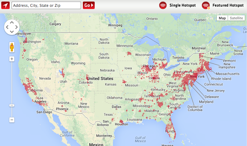
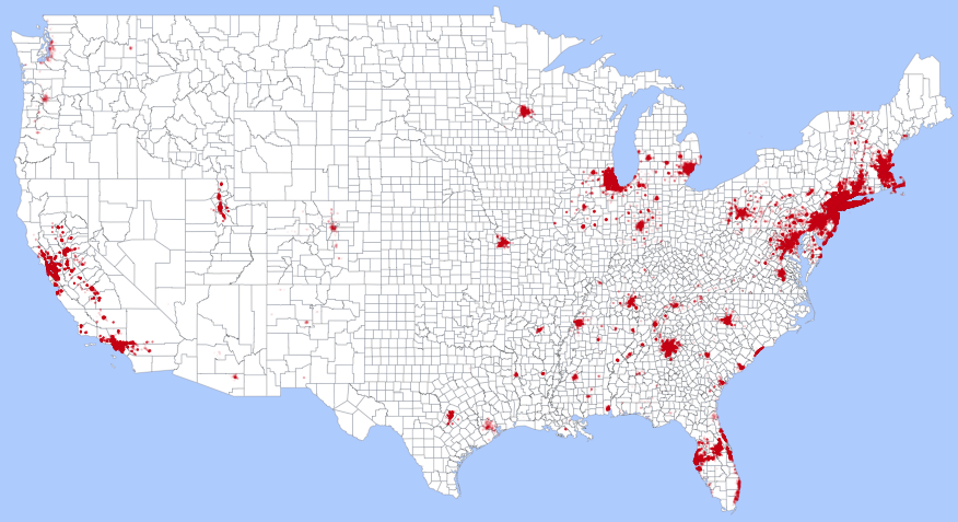
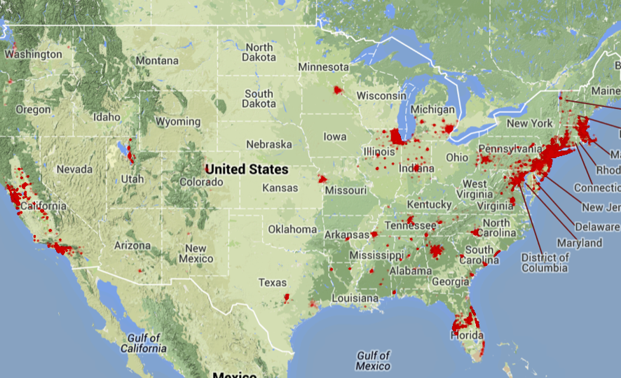
This question has been bugging me since then. As a temporary solution for CrimeMap, I included controls for users to define their own colour scheme. Below are some examples of crime heatmaps that you can create with CrimeMap.


Personally, I really like this feature. I even marketed this as "highly flexible and customisable - colour it the way you like it!" ... I remember saying something like that during LondonR (and I will probably repeat this during useR later).

Then again, the more colours I can use, the more doubts I have with the default Yellow-Red colour scheme. What do others see in those colours? I need to improve on this! In reality, you have one chance, maybe just a few seconds, to tell your very important key messages and to get attention. You can't ask others to tweak the colours of your data visualisation until they get what it means.

Therefore, I know another learning-by-doing journey is required to better understand the use of colours. Only this time, I already have about a year of experience with R under my belt, I decided to capture all the references, thinking and code in one R package.

Existing Tools

Given my poor background in colours, a bit of research on what's available is needed. So far I have found the following. Please suggest other options if you think I should be made aware of (thanks!). I am sure this list will grow as I continue to explore more options.

Online Palette Generator with API

Key R Packages

  • RColorBrewer by Erich Neuwirth - been using this since very first days
  • colorRamps by Tim Keitt - another package that I have been using for a long time
  • colorspace by Ross Ihaka et al. - important package for HCL colours
  • colortools by Gaston Sanchez - for HSV colours
  • munsell by Charlotte Wickham - very useful for exploring and using Munsell colour systems

Funky R Packages and Posts:

Other Languages:


The Plan

"In order to learning something new, find an interesting problem and dive into it!" - This is roughly what Sebastian Thrun said during "Introduction to A.I.", the very first MOOC I participated. It has a really deep impact on me and it has been my motto since then. Fun is key. This project is no exception but I do intend to achieve a bit more this time. Algorithmically, the goal of this mini project can be represented as code below:

> is.fun("my.colours") & is.informative("my.colours")
> TRUE

Seriously speaking, based on the tools and packages mentioned above, I would like to develop a new R package that does the following five tasks. Effectively, these should translate into five key functions (plus a sixth one as a wrapper that goes through all steps in one go).
  1. Extracting colours from images (local or online).
  2. Selecting and (adjusting if needed) colours with web design and colour blindness in mind.
  3. Arranging colours based on colour theory.
  4. Evaluating the aesthetic of a palette systematically (quantifying beauty).
  5. Sharing the palette with friends easily (think the publish( ) and load_gist( ) functions in Shiny, rCharts etc).
I decided to start experimenting with colourful movie posters, especially those from Quentin Tarantino. I love his movies but I also understand that those movies might be offensive to some. That is not my intention here as I just want to bring out the colours. If these examples somehow offend you, please accept my apologies in advance.

First function - rPlotter :: extract_colours( )

The first step is to extract colours from an image. This function is based on dsparks' k-means palettle gist. I modified it slightly to include the excellent EBImage package for easy image processing. For now, I am including this function with my rPlotter package (a package with functions that make plotting in R easier - still in early development).

Note that this is the very first step of the whole process. This function ONLY extracts colours and then returns the colours in simple alphabetical order (of the hex code). The following examples further illustrate why a simple extraction alone is not good enough.

Example One - R Logo

Let's start with the classic R logo.


So three-colour palette looks OK. The colours are less distinctive when we have five colours. For the seven-colour palette, I cannot tell the difference between colours (3) and (5). This example shows that additional processing is needed to rearrange and adjust the colours, especially when you're trying to create a many-colour palette for proper web design and publication.


Example Two - Kill Bill

What does Quentin_Tarantino see in Yellow and Red?


Actually the results are not too bad (at least I can tell the differences).


Example Three - Palette Tarantino

OK, how about a palette set based on some of his movies?


I know more work is needed but for now I am quite happy playing with this.


Example Four - Palette Simpsons

Don't ask why, ask why not ...


I am loving it!


Going Forward

So the above examples show my initial experiments with colours. It will be, to me, a very interesting and useful project in long-term. I look forward to making some sports related data viz when the package reaches a stable version.

The next function in development will be "select_colours()". This will be based on further study on colour theory and other factors like colour blindness. I hope to develop a function that automatically picks the best possible combination of original colours (or adjusts them slightly only if necessary). Once developed, a blog post will follow. Please feel free to fork rPlotter and suggest new functions.

useR! 2014

If you're going to useR! this year, please do come and say hi during the poster session. I will be presenting a poster on the crime maps projects. We can have a chat on CrimeMap, rCrimemap, this colour palette project or any interesting open-source projects.

Acknowledgement

I would like to thank Karthik Ram for developing and sharing the wesanderson package in the first place. I asked him if I could add some more colours to it and he came back with some suggestions. The conversation was followed by some more interesting tweets from Russell Dinnage and Noam Ross. Thank you all!

I would also like to thank Roland Kuhn for showing how to embed individual files of a gist. This is the first time I embed code here properly.

Tweets are the easiest way for me to discuss R these days. Any feedback or suggestion,

To leave a comment for the author, please follow the link and comment on his blog: Blend it like a Bayesian!.

R-bloggers.com offers daily e-mail updates about R news and tutorials on topics such as: visualization (ggplot2, Boxplots, maps, animation), programming (RStudio, Sweave, LaTeX, SQL, Eclipse, git, hadoop, Web Scraping) statistics (regression, PCA, time series, trading) and more...

How Do Cities Feel?

$
0
0

(This article was first published on Ripples, and kindly contributed to R-bloggers)

If you are lost and feel alone, circumnavigate the globe (For You, Coldplay)

You can not consider yourself a R-blogger until you do an analysis of Twitter using twitteR package. Everybody knows it. So here I go.

Inspired by the fabulous work of Jonathan Harris I decided to compare human emotions of people living (or twittering in this case) in different cities. My plan was analysing tweets generated in different locations of USA and UK with one thing in common: all of them must contain the string “I FEEL”. These are the main steps I followed:

  • Locate cities I want to analyze using world cities database of maps package
  • Download tweets around these locations using searchTwitter function of twitteR package.
  • Cross tweets with positive and negative lists of words and calculate a simple scoring for each tweet as number of positive words – number of negative words
  • Calculate how many tweets have non-zero scoring; since these tweets put into words some emotion I call them sentimental tweets
  • Represent cities in a bubble chart where x-axis is percentage of sentimental tweets, y-axis is average scoring and size of bubble is population

This is the result of my experiment:HowDoCitiesFeel3

These are my conclusions (please, do not take it seriously):

  • USA cities seem to have better vibrations and are more sentimental than UK ones
  • Capital city is the happiest one for both countries
  • San Francisco (USA) is the most sentimental city of the analysis; on the other hand, Liverpool (UK) is the coldest one
  • The more sentimental, the better vibrations

From my point of view, this analysis has some important limitations:

  • It strongly depends on particular events (i.e. local football team wins the championship)
  • I have no idea of what kind of people is behind tweets
  • According to my experience, searchTwitter only works well for a small number of searches (no more than 300); for larger number of tweets to return, it use to give malformed JSON response error from server

Anyway, I hope it will serve as starting point of some other analysis in the future. At least, I learned interesting things about R doing it.

Here you have the code:

library(twitteR)
library(RCurl)
library(maps)
library(plyr)
library(stringr)
library(bitops)
library(scales)
#Register
if (!file.exists('cacert.perm'))
{
  download.file(url = 'http://curl.haxx.se/ca/cacert.pem', destfile='cacert.perm')
}
requestURL="https://api.twitter.com/oauth/request_token"
accessURL="https://api.twitter.com/oauth/access_token"
authURL="https://api.twitter.com/oauth/authorize"
consumerKey = "YOUR CONSUMER KEY HERE"
consumerSecret = "YOUR CONSUMER SECRET HERE"
Cred <- OAuthFactory$new(consumerKey=consumerKey,
                         consumerSecret=consumerSecret,
                         requestURL=requestURL,
                         accessURL=accessURL,
                         authURL=authURL)
Cred$handshake(cainfo=system.file("CurlSSL", "cacert.pem", package="RCurl"))
#Save credentials
save(Cred, file="twitter authentification.Rdata")
load("twitter authentification.Rdata")
registerTwitterOAuth(Cred)
options(RCurlOptions = list(cainfo = system.file("CurlSSL", "cacert.pem", package = "RCurl")))
#Cities to analyze
cities=data.frame(
  CITY=c('Edinburgh', 'London', 'Glasgow', 'Birmingham', 'Liverpool', 'Manchester',
         'New York', 'Washington', 'Las Vegas', 'San Francisco', 'Chicago','Los Angeles'),
  COUNTRY=c("UK", "UK", "UK", "UK", "UK", "UK", "USA", "USA", "USA", "USA", "USA", "USA"))
data(world.cities)
cities2=world.cities[which(!is.na(match(
str_trim(paste(world.cities$name, world.cities$country.etc, sep=",")),
str_trim(paste(cities$CITY, cities$COUNTRY, sep=","))
))),]
cities2$SEARCH=paste(cities2$lat, cities2$long, "10mi", sep = ",")
cities2$CITY=cities2$name
#Download tweets
tweets=data.frame()
for (i in 1:nrow(cities2))
{
  tw=searchTwitter("I FEEL", n=400, geocode=cities2[i,]$SEARCH)
  tweets=rbind(merge(cities[i,], twListToDF(tw),all=TRUE), tweets)
}
#Save tweets
write.csv(tweets, file="tweets.csv", row.names=FALSE)
#Import csv file
city.tweets=read.csv("tweets.csv")
#Download lexicon from http://www.cs.uic.edu/~liub/FBS/opinion-lexicon-English.rar
hu.liu.pos = scan('lexicon/positive-words.txt',  what='character', comment.char=';')
hu.liu.neg = scan('lexicon/negative-words.txt',  what='character', comment.char=';')
#Function to clean and score tweets
score.sentiment=function(sentences, pos.words, neg.words, .progress='none')
{
  require(plyr)
  require(stringr)
  scores=laply(sentences, function(sentence, pos.word, neg.words) {
    sentence=gsub('[[:punct:]]','',sentence)
    sentence=gsub('[[:cntrl:]]','',sentence)
    sentence=gsub('\\d+','',sentence)
    sentence=tolower(sentence)
    word.list=str_split(sentence, '\\s+')
    words=unlist(word.list)
    pos.matches=match(words, pos.words)
    neg.matches=match(words, neg.words)
    pos.matches=!is.na(pos.matches)
    neg.matches=!is.na(neg.matches)
    score=sum(pos.matches) - sum(neg.matches)
    return(score)
  }, pos.words, neg.words, .progress=.progress)
  scores.df=data.frame(score=scores, text=sentences)
  return(scores.df)
}
cities.scores=score.sentiment(city.tweets[1:nrow(city.tweets),], hu.liu.pos, hu.liu.neg, .progress='text')
cities.scores$pos2=apply(cities.scores, 1, function(x) regexpr(",",x[2])[1]-1)
cities.scores$CITY=apply(cities.scores, 1, function(x) substr(x[2], 1, x[3]))
cities.scores=merge(x=cities.scores, y=cities, by='CITY')
df1=aggregate(cities.scores["score"], by=cities.scores[c language="("CITY")"][/c], FUN=length)
names(df1)=c("CITY", "TWEETS")
cities.scores2=cities.scores[abs(cities.scores$score)>0,]
df2=aggregate(cities.scores2["score"], by=cities.scores2[c language="("CITY")"][/c], FUN=length)
names(df2)=c("CITY", "TWEETS.SENT")
df3=aggregate(cities.scores2["score"], by=cities.scores2[c language="("CITY")"][/c], FUN=mean)
names(df3)=c("CITY", "TWEETS.SENT.SCORING")
#Data frame with results
df.result=join_all(list(df1,df2,df3,cities2), by = 'CITY', type='full')
#Plot results
radius <- sqrt(df.result$pop/pi)
symbols(100*df.result$TWEETS.SENT/df.result$TWEETS, df.result$TWEETS.SENT.SCORING, circles=radius,
        inches=0.85, fg="white", bg="gold", xlab="Sentimental Tweets", ylab="Scoring Of Sentimental Tweets (Average)",
        main="How Do Cities Feel?")
text(100*df.result$TWEETS.SENT/df.result$TWEETS, df.result$TWEETS.SENT.SCORING, paste(df.result$CITY, df.result$country.etc, sep="-"), cex=1, col="gray50")

To leave a comment for the author, please follow the link and comment on his blog: Ripples.

R-bloggers.com offers daily e-mail updates about R news and tutorials on topics such as: visualization (ggplot2, Boxplots, maps, animation), programming (RStudio, Sweave, LaTeX, SQL, Eclipse, git, hadoop, Web Scraping) statistics (regression, PCA, time series, trading) and more...

Can You Track Me Now? (Visualizing Xfinity Wi-Fi Hotspot Coverage) [Part 1]

$
0
0

(This article was first published on Data Driven Security, and kindly contributed to R-bloggers)

This is the first of a two-part series. Part 1 sets up the story and goes into how to discover, digest & reformat the necessary data. Part 2 will show how to perform some basic visualizations and then how to build beautiful & informative density maps from the data and offer some suggestions as to how to prevent potential tracking.

Xfinity has a Wi-Fi hotspot offering that they offer through a partnership with BSG Wireless. Customers of Xfinity get access to the hotspots for “free” and you can pay for access to them if you aren’t already a customer. I used the service a while back in near area where I live (which is just southwest of the middle of nowhere) when I needed internet access and 3G/4G connectivity was non-existent.

Since that time, I started noticing regular associations to Xfinity hotspots and also indicators saying it was available (i.e. when Wi-Fi was “off” on my phone but not really off). When driving, that caused some hiccups with streaming live audio since I wasn’t in a particular roaming area long enough to associate and grab data, but was often in range just long enough to temporarily disrupt the stream.

On a recent family+school trip to D.C., I noticed nigh pervasive coverage of Xfinity Wi-Fi as we went around the sights (with varied levels of efficacy when connecting to them). That finally triggered a “Hrm. Somewhere in their vast database, they know I was in Maine a little while ago and now am in D.C.”. There have been plenty of articles over the years on the privacy issues of hotspots, but this made me want to dig into just how pervasive the potential for tracking was on Xfinity Wi-Fi.

DISCLAIMER I have no proof—nor am I suggesting—that Xfinity or BSG Wireless is actually maintaining records of associations or probes from mobile devices. However, the ToS & privacy pages on each of their sites did not leave me with any tpye of warm/fuzzy feeling that this data is not—in fact—being used for tracking purposes.

Digging for data

Since the Xfinity Wi-Fi site suggests using their mobible app to find hotspots, I decided to grab it for both my iPhone & Galaxy S3 and see what type of data might be available. I first zoomed out to the seacoast region to get a feel for the Xfinity Wi-Fi coverage:

Yikes! If BSG (or any similar service) is, indeed, recording all associations & probes, it looks like there’s almost nowhere to go in the seacoast area without being tracked.

Not wanting to use a tiny screen to continue my investigations, I decided to poke around the app a bit to see if there might be any way to get the locations of the hotspots to work with in R. Sure enough, there was:

I fired up Burp Proxy, reconfigured my devices to use it and recorded session as I poked around the mobile app/tool. There were “are you there?” checks before almost every API call, but I was able to see calls to a “discovery” service as well as the URLs for the region datasets.

The following Burp Proxy intercept shows that the app requesting data from the “discovery” API and receiving a JSON response:

REQUEST

(Host: http://datafeed.bsgwireless.com)

POST /ajax/finderDataService/discover.php HTTP/1.1
Accept-Encoding: gzip,deflate
Content-Length: 40
Content-Type: application/x-www-form-urlencoded
Host: datafeed.bsgwireless.com
Connection: Keep-Alive

api_key=API_KEY_STRING_FROM_BURP_INTERCEPT

RESPONSE

HTTP/1.1 200 OK
Date: Sat, 31 May 2014 16:20:41 GMT
Server: Apache/2.2.22 (Debian)
X-Powered-By: PHP/5.4.4-14+deb7u9
Set-Cookie: PHPSESSID=mci434v907571ihq7d16vtmce0; path=/
Expires: Thu, 19 Nov 1981 08:52:00 GMT
Cache-Control: no-store, no-cache, must-revalidate, post-check=0, pre-check=0
Pragma: no-cache
Vary: Accept-Encoding
Content-Length: 1306
Keep-Alive: timeout=5, max=100
Connection: Keep-Alive
Content-Type: text/html
        {"success":true,"results":{"baseURL":"http:\/\/comcast.datafeed.bsgwireless.com\/data\/comcast","fileList":[{"id":"45","name":"metadata.sqlite","title":"Metadata","description":null,"lastUpdated":"20140513","fileSize":"11264","txSize":"3210","isMeta":true},{"id":"51","name":"finder_comcast_matlantic.sqlite","title":"Mid-Atlantic","description":"DC, DE, MD, NJ, PA, VA, WV","lastUpdated":"20140513","fileSize":"9963520","txSize":"2839603","isMeta":false},{"id":"52","name":"finder_comcast_west.sqlite","title":"West","description":"AK, AZ, CA, CO, HI, ID, MT, NV, NM, ND, OR, SD, UT, WA, WY","lastUpdated":"20140513","fileSize":"5770240","txSize":"1644518","isMeta":false},{"id":"53","name":"finder_comcast_midwest.sqlite","title":"Midwest","description":"AR, IL, IN, IA, KS, KY, MI, MN, MO, NE, OH, OK, WI","lastUpdated":"20140513","fileSize":"3235840","txSize":"922214","isMeta":false},{"id":"54","name":"finder_comcast_nengland.sqlite","title":"Northeast","description":"CT, ME, MA, NH, NY, RI, VT","lastUpdated":"20140513","fileSize":"10811392","txSize":"3081246","isMeta":false},{"id":"55","name":"finder_comcast_south.sqlite","title":"South","description":"AL, FL, GA, LA, MS, NC, SC, TN, TX","lastUpdated":"20140513","fileSize":"5476352","txSize":"1560760","isMeta":false}],"generated":1401553245}}

We can use R to make the same request and also turn the JSON into R objects that we can work with via the jsonlite library:

library(RCurl)
library(jsonlite)

# post the same form/query via RCurl

resp <- postForm("http://datafeed.bsgwireless.com/ajax/finderDataService/discover.php", 
                 api_key="API_KEY_STRING_FROM_BURP_INTERCEPT")

# convert the JSON response to R objects

resp <- fromJSON(as.character(resp))

# take a peek at what we've got

print(resp)
## $success
## [1] TRUE
## 
## $results
## $results$baseURL
## [1] "http://comcast.datafeed.bsgwireless.com/data/comcast"
## 
## $results$fileList
##   id                            name        title
## 1 45                 metadata.sqlite     Metadata
## 2 51 finder_comcast_matlantic.sqlite Mid-Atlantic
## 3 52      finder_comcast_west.sqlite         West
## 4 53   finder_comcast_midwest.sqlite      Midwest
## 5 54  finder_comcast_nengland.sqlite    Northeast
## 6 55     finder_comcast_south.sqlite        South
##                                                  description lastUpdated
## 1                                                       <NA>    20140513
## 2                                 DC, DE, MD, NJ, PA, VA, WV    20140513
## 3 AK, AZ, CA, CO, HI, ID, MT, NV, NM, ND, OR, SD, UT, WA, WY    20140513
## 4         AR, IL, IN, IA, KS, KY, MI, MN, MO, NE, OH, OK, WI    20140513
## 5                                 CT, ME, MA, NH, NY, RI, VT    20140513
## 6                         AL, FL, GA, LA, MS, NC, SC, TN, TX    20140513
##   fileSize  txSize isMeta
## 1    11264    3210   TRUE
## 2  9963520 2839603  FALSE
## 3  5770240 1644518  FALSE
## 4  3235840  922214  FALSE
## 5 10811392 3081246  FALSE
## 6  5476352 1560760  FALSE
## 
## $results$generated
## [1] 1401553861

We can see that each region (from the app screen capture) has an entry in the resp$results$fileList data frame that obviously corresponds to a SQLite database for that region. Furthermore, each one also shows when it was last updated (which you can then use to determine if you need to re-download it). There’s also a metadata.sqlite file that might be interesting to poke around at as well.

The API also gives us the base URL which matches the request from the Burp Proxy session (when retrieving an individal dataset file). The following is the Burp Proxy request capture from the iOS app:

GET /data/comcast/finder_comcast_nengland.sqlite HTTP/1.1
Host: comcast.datafeed.bsgwireless.com
Pragma: no-cache
Proxy-Connection: keep-alive
Accept: */*
User-Agent: XFINITY%20WiFi/232 CFNetwork/672.1.14 Darwin/14.0.0
Accept-Language: en-us
Accept-Encoding: gzip
Connection: keep-alive

The Android version of the app sends somewhat different request headers, including an Authorization header that Base64 decodes to csl:123456 (and isn’t used by the API):

GET /data/comcast/finder_comcast_midwest.sqlite HTTP/1.1
Accept-Encoding: gzip
Host: comcast.datafeed.bsgwireless.com
Connection: Keep-Alive
User-Agent: Apache-HttpClient/UNAVAILABLE (java 1.4)
Authorization: Basic Y3NsOjEyMzQ1Ng==

Given that there are no special requirements for downloading the data files (even the User-Agent isn’t standardized between operating system versions), we can use plain ol’ download.file from the “built-in” utils package to handle retrieval:

# plyr isn't truly necessary, but I like the syntax standardization it provides

library(plyr)

l_ply(resp$results$fileList$name, function(x) {
  download.file(sprintf("http://comcast.datafeed.bsgwireless.com/data/comcast/%s", x),
                sprintf("data/%s",x))
})

NOTE: As you can see in the example, I’m storing all the data files in a data subdirectory of the project I started for this exaple.

While the metadata.sqlite file is interesting, the data really isn’t all that useful for this post since the Xfinity app doesn’t use most of it (and is very US-centric). I suspect that data is far more interesting in the full BSG hotspot data set (which we aren’t using here). Therefore, we’ll just focus on taking a look at the hotspot data, specifically the sites table:

CREATE TABLE "sites" (
  "siteUID"               integer PRIMARY KEY NOT NULL DEFAULT null, 
  "siteTypeUID"           integer NOT NULL DEFAULT null,
  "siteCategory"          integer DEFAULT null, 
  "siteName"              varchar NOT NULL DEFAULT null, 
  "address1"              varchar DEFAULT null, 
  "address2"              varchar DEFAULT null, 
  "town"                  varchar,
  "county"                varchar, 
  "postcode"              varchar, 
  "countryUID"            integer DEFAULT null, 
  "latitude"              double NOT NULL, 
  "longitude"             double NOT NULL, 
  "siteDescription"       text DEFAULT null, 
  "siteWebsite"           varchar DEFAULT null, 
  "sitePhone"             varchar DEFAULT null, 
  "operatorUID"           integer NOT NULL DEFAULT null, 
  "ssid"                  varchar(50), 
  "connectionTypeUID"     integer DEFAULT null, 
  "serviceProviderBrand"  varchar(50) DEFAULT null, 
  "additionalSearchTerms" varchar);

You can get an overview on how to use the SQLite command line tool in the SQLite CLI documentation if you’re unfamiliar with SQL/SQLite.

The app most likely uses individual databases to save device space and bandwith, but it would be helpful if we had all the hotspot data in one data frame. We can do this pretty easily in R since we can work with SQLite databases via the RSQLite package and use ldply to combine results for us:

library(RSQLite)
library(sqldf)

# the 'grep' is here since we don't want to process the 'metadata' file

xfin <- ldply(grep("metadata.sqlite", 
                   resp$results$fileList$name, 
                   invert=TRUE, value=TRUE), function(x) {

  db <- dbConnect(SQLite(), dbname=sprintf("data/%s", x))

  query <- "SELECT siteCategory, siteName, address1,  town, county, 
                   postcode, latitude, longitude, siteWebsite, sitePhone
            FROM sites"

  results <- dbSendQuery(db, query)

  # this makes a data frame from the entirety of the results

  aps <- fetch(results, -1)

  # the operation can take a little while, so this just shows progress
  # and also whether we retrieved all the results from the query for each call
  # by using message() you can use suppressMessages() to disable the
  # "debugging" messages

  message("Loading [", x, "]... ", ifelse(dbHasCompleted(results), "successful!", "unsuccessful :-("))

  dbClearResult(results)

  return(aps)

})

I had intended to use more than just latitude & longitude with this post, but ended up not using it. I left it in the query since a future post might use it and also as an example for those unfamiliar with using SQLite/RSQLite.

The function in the ldply combines each region’s data frame into one. We can get a quick overview of what it looks like:

str(xfin) 
## 'data.frame':    261365 obs. of  10 variables:
##  $ siteCategory: int  2 2 2 2 2 2 2 2 3 2 ...
##  $ siteName    : chr  "CableWiFi" "CableWiFi" "CableWiFi" "CableWiFi" ...
##  $ address1    : chr  "7 ELM ST" "603 BROADWAY" "6501 HUDSON AVE" "1607 CORLIES AVE" ...
##  $ town        : chr  "Morristown" "Bayonne" "West New York" "Neptune" ...
##  $ county      : chr  "New Jersey" "New Jersey" "New Jersey" "New Jersey" ...
##  $ postcode    : chr  "07960" "07002" "07093" "07753" ...
##  $ latitude    : num  40.8 40.7 40.8 40.2 40.9 ...
##  $ longitude   : num  -74.5 -74.1 -74 -74 -74.6 ...
##  $ siteWebsite : chr  "" "" "" "" ...
##  $ sitePhone   : chr  "" "" "" "" ...

Now that we have the data into the proper format, we’ll cover how to visualize it in the second and final part of the series.

To leave a comment for the author, please follow the link and comment on his blog: Data Driven Security.

R-bloggers.com offers daily e-mail updates about R news and tutorials on topics such as: visualization (ggplot2, Boxplots, maps, animation), programming (RStudio, Sweave, LaTeX, SQL, Eclipse, git, hadoop, Web Scraping) statistics (regression, PCA, time series, trading) and more...

Proficiency levels @ PISA and visualisation challenge @ useR!2014

$
0
0

(This article was first published on SmarterPoland » PISA in english, and kindly contributed to R-bloggers)

16 days to go for submissions in the DataVis contest at useR!2014 (see contest webpage).
The contest is focused on PISA data and students’ skills. The main variables that reflect pupil skills in math / reading / science are plausible values e.g. columns PV1MATH, PV1READ, PV1SCIE in the dataset.
But, these values are normalized to have mean 500 and sd 100. And it is not that easy to understand what the skill level 600 means and is 12 points in average a big difference. To overcome this PISA has introduced seven proficiency levels (from 0 to 6, see http://nces.ed.gov/pubs2014/2014024_tables.pdf) that base on plausible values with cutoffs 358, 420, 482, 545, 607, 669.
It is assumed that, for example, at level 6 ,,students can conceptualize, generalize, and utilize information based on their investigations and modeling of complex problem situations, and can use their knowledge in relatively non-standard contexts”.

So, instead of looking at means we can now take a look at fractions of students at given proficiency level. To have some fun we use sp and rworldmap and RColorBrewer packages to have country shapes instead of bars and dots that are supposed to represent pupils that take part in the study. The down side is that area does not correspond to height so it might be confusing. We add horizontal lines to expose the height.


And here is the R code

library(ggplot2)
library(reshape2)
library(rworldmap)
library(RColorBrewer)
map.world <- map_data(map = "world")
cols <- brewer.pal(n=7, "PiYG")
 
# read students data from PISA 2012
# directly from URL
con <- url("http://beta.icm.edu.pl/PISAcontest/data/student2012.rda")
load(con)
prof.scores <- c(0, 358, 420, 482, 545, 607, 669, 1000)
prof.levels <- cut(student2012$PV1MATH, prof.scores, paste("level", 1:7))
 
plotCountry <- function(cntname = "Poland", cntname2 = cntname) {
  props <- prop.table(tapply(student2012$W_FSTUWT[student2012$CNT == cntname],
         prof.levels[student2012$CNT == cntname], 
         sum))
  cntlevels <- rep(1:7, times=round(props*5000))
  cntcontour <- map.world[map.world$region == cntname2,]
  cntcontour <- cntcontour[cntcontour$group == names(which.max(table(cntcontour$group))), ]
  wspx <- range(cntcontour[,1])
  wspy <- range(cntcontour[,2])
  N <- length(cntlevels)
  px <- runif(N) * diff(wspx) + wspx[1]
  py <- sort(runif(N) * diff(wspy) + wspy[1])
  sel <- which(point.in.polygon(px, py, cntcontour[,1], cntcontour[,2], mode.checked=FALSE) == 1)
  df <- data.frame(long = px[sel], lat = py[sel], level=cntlevels[sel])  
  par(pty="s", mar=c(0,0,4,0))
  plot(df$long, df$lat, col=cols[df$level], pch=19, cex=3,
       bty="n", xaxt="n", yaxt="n", xlab="", ylab="")
}
 
par(mfrow=c(1,7))
#
# PISA and World maps are using differnt country names,
# thus in some cases we need to give two names
plotCountry(cntname = "Korea", cntname2 = "South Korea")
plotCountry(cntname = "Japan", cntname2 = "Japan")
plotCountry(cntname = "Finland")
plotCountry(cntname = "Poland")
plotCountry(cntname = "France", cntname2 = "France")
plotCountry(cntname = "Italy", cntname2 = "Italy")
plotCountry(cntname = "United States of America", cntname2 = "USA")

To leave a comment for the author, please follow the link and comment on his blog: SmarterPoland » PISA in english.

R-bloggers.com offers daily e-mail updates about R news and tutorials on topics such as: visualization (ggplot2, Boxplots, maps, animation), programming (RStudio, Sweave, LaTeX, SQL, Eclipse, git, hadoop, Web Scraping) statistics (regression, PCA, time series, trading) and more...

Can You Track Me Now? (Visualizing Xfinity Wi-Fi Hotspot Coverage) [Part 2]

$
0
0

(This article was first published on Data Driven Security, and kindly contributed to R-bloggers)

This is the second of a two-part series. Part 1 set up the story and goes into how to discover, digest & reformat the necessary data. This concluding segment will show how to perform some basic visualizations and then how to build beautiful & informative density maps from the data and offer some suggestions as to how to prevent potential tracking.

I’ll start with the disclaimer from the previous article:

DISCLAIMER I have no proof—nor am I suggesting—that Xfinity or BSG Wireless is actually maintaining records of associations or probes from mobile devices. However, the ToS & privacy pages on each of their sites did not leave me with any tpye of warm/fuzzy feeling that this data is not—in fact—being used for tracking purposes.

Purely by coincidence, @NPRNewsSteve Henn also decided to poke at Wi-Fi networks during their cyber series this week and noted other potential insecurities of Comcast’s hotspot network. That means along with tracking, you could also be leaking a great deal of information as you go from node to node. Let’s see just how pervasive these nodes are.

Visualizing Hotspots

Now, you don’t need the smartphone app to see the hotspots. Xfinity has a web-based hotspot finder based on Google Maps:

Those “dots” are actually bitmap tiles (even as you zoom in). Xfinity either did that to “protect” the data, save bandwidth or speed up load-time (creating 260K+ points can take a few, noticeable seconds). We can reproduce this in R without (and with) Google Maps pretty easily:

library(maptools)
library(maps)
library(rgeos)
library(ggcounty)

# you can grab ggcounty via:
# install.packages("devtools")
# install_github("hrbrmstr/ggcounty")

# grab the US map with counties

us <- ggcounty.us(color="#777777", size=0.125)

# plot the points in "Xfinity red" with a 
# reasonable alpha setting & point size

gg <- us$gg
gg <- gg %+% xfin + aes(x=longitude, y=latitude)
gg <- gg + geom_point(color="#c90318", size=1, alpha=1/20)
gg <- gg + coord_map(projection="mercator")
gg <- gg + xlim(range(us$map$long))
gg <- gg + ylim(range(us$map$lat))
gg <- gg + labs(x="", y="")
gg <- gg + theme_bw()

# the map tends to stand out beter on a non-white background
# but the panel background color isn't truly "necessary"

gg <- gg + theme(panel.background=element_rect(fill="#878787"))
gg <- gg + theme(panel.grid=element_blank())
gg <- gg + theme(panel.border=element_blank())
gg <- gg + theme(axis.ticks.x=element_blank())
gg <- gg + theme(axis.ticks.y=element_blank())
gg <- gg + theme(axis.text.x=element_blank())
gg <- gg + theme(axis.text.y=element_blank())
gg <- gg + theme(legend.position="none")
gg

library(ggmap)

x_map <- get_map(location = 'united states', zoom = 4, maptype="terrain", source = 'google')
xmap_gg <- ggmap(x_map)

gg <- xmap_gg %+% xfin + aes(x=longitude, y=latitude)
gg <- gg %+% xfin + aes(x=longitude, y=latitude)
gg <- gg + geom_point(color="#c90318", size=1.5, alpha=1/50)
gg <- gg + coord_map(projection="mercator")
gg <- gg + xlim(range(us$map$long))
gg <- gg + ylim(range(us$map$lat))
gg <- gg + labs(x="", y="")
gg <- gg + theme_bw()
gg <- gg + theme(panel.grid=element_blank())
gg <- gg + theme(panel.border=element_blank())
gg <- gg + theme(axis.ticks.x=element_blank())
gg <- gg + theme(axis.ticks.y=element_blank())
gg <- gg + theme(axis.text.x=element_blank())
gg <- gg + theme(axis.text.y=element_blank())
gg <- gg + theme(legend.position="none")
gg

It’s a bit interesting that they claim over a million hotspots but the database has less then 300K entries.

I made the dots a bit smaller and used a fairly reasonable alpha setting for them. However, the macro- (i.e. the view of the whole U.S.) plus dot-view really doesn’t give a good feel for the true scope of the coverage (or possible tracking). For that, we can turn to state-based density maps.

There are many ways to generate/display density maps. Since we’ll still want to display the individual hotspot points as well as get a feel for the area, we’ll use one that outlines and gradient fills in the regions, then plot the individual points on top of them.

library(ggcounty)

l_ply(grep("Idaho", unique(xfin$county), value=TRUE, invert=TRUE), function(state) {

  print(state) # lets us know progress as this takes a few seconds/state

  gg.c <- ggcounty(state, color="#737373", fill="#f0f0f0", size=0.175)

  gg <- gg.c$gg
  gg <- gg %+% xfin[xfin$county==state,] + aes(x=longitude, y=latitude)
  gg <- gg + stat_density2d(aes(fill=..level.., alpha=..level..), 
                            size=0.01, bins=100, geom='polygon')
  gg <- gg + scale_fill_gradient(low="#fddbc7", high="#67001f")
  gg <- gg + scale_alpha_continuous(limits=c(100), 
                                    breaks=seq(0, 100, by=1.0), guide=FALSE)
  gg <- gg + geom_density2d(color="#d6604d", size=0.2, alpha=0.5, bins=100)
  gg <- gg + geom_point(color="#1a1a1a", size=0.5, alpha=1/30)
  gg <- gg + coord_map(projection="mercator")
  gg <- gg + xlim(range(gg.c$map$long))
  gg <- gg + ylim(range(gg.c$map$lat))
  gg <- gg + labs(x="", y="")
  gg <- gg + theme_bw()
  gg <- gg + theme(panel.grid=element_blank())
  gg <- gg + theme(panel.border=element_blank())
  gg <- gg + theme(axis.ticks.x=element_blank())
  gg <- gg + theme(axis.ticks.y=element_blank())
  gg <- gg + theme(axis.text.x=element_blank())
  gg <- gg + theme(axis.text.y=element_blank())
  gg <- gg + theme(legend.position="none")

  ggsave(sprintf("output/%s.svg", gsub(" ", "", state)), gg, width=8, height=8, units="in", dpi=140)
  ggsave(sprintf("output/%s.png", gsub(" ", "", state)), gg, width=6, height=6, units="in", dpi=140)

})

The preceeding code will produce a density map per state. Below is an abbreviated gallery of (IMO) the most interesting states. You can click on each for a larger (SVG) version.

Some of SVGs have a hefty file size, so they might take a few seconds to load.


You can also single out your own state for examination:

Now, these are just basic density maps. They don’t take into account Wi-Fi range, so the areas are larger than actual signal coverage. The purpose was to show just how widespread (or minimal) the coverage is vs convey discrete tracking precision. As you jump from association to association, it would be trivial for any provider to “connect the dots”.

Covering Your Tracks

Comcast (Xfinity) and AT&T aren’t the only places where this tracking can occur. CreepyDOL was demoed at BlackHat in 2013 (making it pretty simple for almost anyone to setup tracking). Stores already use your Wi-Fi associations to track you. Navizon has a whole product/service based on the concept.

Apple is trying to help with a new feature in iOS 8 that will randomize MAC addresses when probing for access points and David Schuetz has advocated deleting preferred networks from your iOS networks list.

What can you do while you wait for iOS (and wait even longer for the framented Android world to catch up)? Android users can give AVG’s new PrivacyFix a go, but one of your only direct controls is to disable Wi-Fi, but that might not truly help if your mobile operating system does not deal well with passive Wi-Fi probes. Another option (as mentioned above) is to regularly purge the list of previously associated networks. You could even go so far as to bundle up your phone and stop all signales coming in and out, but that somewhat defeats the purpose of having your mobile with you.

Remain aware that the tracking can happen invisibly anywhere and, perhaps more importantly, the dangers that open Wi-Fi networks pose in general. Use a VPN service like Cloak to at least ensure all your transmissions are free from local prying eyes so the trackers have as little data to associate with you as possible.

Finally, keep putting pressure on the FTC to help with this privacy issue. While FTC/FCC efforts won’t stop malicious actors, it might help reign in businesses and encourage more privacy innovation on the part of Apple/Android/Microsoft.

To leave a comment for the author, please follow the link and comment on his blog: Data Driven Security.

R-bloggers.com offers daily e-mail updates about R news and tutorials on topics such as: visualization (ggplot2, Boxplots, maps, animation), programming (RStudio, Sweave, LaTeX, SQL, Eclipse, git, hadoop, Web Scraping) statistics (regression, PCA, time series, trading) and more...

Identifying Pathways in the Consumer Decision Journey: Nonnegative Matrix Factorization

$
0
0

(This article was first published on Engaging Market Research, and kindly contributed to R-bloggers)
The Internet has freed us from the shackles of the yellow page directory, the trip to the nearby store to learn what is available, and the forced choice among a limited set of alternatives. The consumer is in control of their purchase journey and can take any path they wish. But do they? It's a lot of work for our machete-wielding consumer cutting their way through the product jungle. The consumer decision journey is not an itinerary, but neither is it aimless meandering. Perhaps we do not wish to follow the well-worn trail laid out by some marketing department. The consumer is free to improvise, not by going where no one has gone before, but by creating personal variation using a common set of journey components shared with others.

Even with all the different ways to learn about products and services, we find constraints on the purchase process with some touchpoint combinations more likely than others. For example, one could generate a long list of all the possible touchpoints that might trigger interest, provide information, make recommendations, and enable purchase. Yet, we would expect any individual consumer to encounter only a small proportion of this long list. A common journey might be no more than a seeing an ad followed by a trip to a store. For frequently purchased products, the entire discovery-learning-comparing-purchase process could collapse into a single point-of-sale (PoS) touchpoint, such as product packaging on a retail shelf.

The figure below comes from a touchpoint management article discussing the new challenges of online marketing. This example was selected because it illustrates how easy it is to generate touchpoints as we think of all the ways that a consumer interacts with or learns about a product. Moreover, we could have been much more detailed because episodic memory allows us to relive the product experience (e.g., the specific ads seen, the packaging information attended to, the pages of the website visited). The touchpoint list quickly gets lengthy, and the data matrix becomes sparser because an individual consumer is not likely to engage intensively with many products. The resulting checklist dataset is a high-dimensional consumer-by-touchpoint matrix with lots of columns and cells containing some ones but mostly zeroes.


It seems natural to subdivide the columns into separate modes of interaction as shown by the coloring in the above figure (e.g., POS, One-to-One, Indirect, and Mass). It seems natural because different consumers rely on different modes to learn and interact with product categories. Do you buy by going to the store and selecting the best available product, or do you search and order online without any physical contact with people or product? Like a Rubik's cube, we might be able to sort rows and columns simultaneously so that the reordered matrix would appear to be block diagonal with most of the ones within the blocks and most of the zeroes outside. You can find an illustration in a previous post on the reorderable data matrix. As we shall see later, nonnegative matrix factorization "reorders" indirectly by excluding negative entries in the data matrix and its factors. A more direct approach to reordering would use the R packages for biclustering or seriation. Both of these links offer different perspectives on how to cluster or order rows and columns simultaneously.

Nonnegative Matrix Factorization (NMF) with Simulated Data

I intend to rely on the R package NMF and a simulated data set based on the above figure. I will keep it simple and assume only two pathways: an online journey through the 10 touchpoints marked with an "@" in the above figure and an offline journey through the remaining 20 touchpoints. Clearly, consumers are more likely to encounter some touchpoints more often than others, so I have made some reasonable but arbitrary choices. The R code at the end of this post reveals the choices that were made and how I generated the data using the sim.rasch function from the psych R package. Actually, all you need to know is that the dataset contains 400 consumers, 200 interacting more frequently online and 200 with greater offline contact. I have sorted the 30 touchpoints from the above figure so that the first 10 are online (e.g., search engine, website, user forum) and the last 20 are offline (e.g., packaging information, ad in magazine, information display). Although the patterns within each set of online and offline touchpoints are similar, the result is two clearly different pathways as shown by the following plot.


It should be noted that the 400 x 30 data matrix contained mostly zeroes with only 11.2% of the 12,000 cells indicating any contact. Seven of the respondents did not indicate any interaction at all and were removed from the analysis. The mode was 3 touchpoints per consumer, and no one reported more than 11 interactions (although the verb "reported" might not be appropriate to describe simulated data).

If all I had was the 400 respondents, how would I identify the two pathways? Actually, k-means often does quite well, but not in this case with so many infrequent binary variables. Although using the earlier mentioned biclustering approach in R, Dolnicar and her colleagues will help us understand the problems encounters when conducting market segmentation with high-dimensional data. When asked to separate the 400 into two groups, k-means clustering was able to identify correctly only 55.5% of the respondents. Before we overgeneralize, let me note that k-means performed much better when the proportions were higher (e.g., raise both lines so that they peak above 0.5 instead of below 0.4), although that is not much help with high-dimensional scare data.

And, what about NMF? I will start with the results so that you will be motivated to remain for the explanation in the next section. Overall, NMF placed correctly 81.4% of the respondents, 85.9% of the offline segment and 76.9% of the online segment. In addition, NMF extracted two latent variables that separated the 30 touchpoints into the two sets of 10 online and 20 offline interactions.

So, what is nonnegative matrix factorization?

Have you run or interpreted a factor analysis? Factor analysis is matrix factorization where the correlation matrix R is factored into factor loadings: R = FF'. Structural equation modeling is another example of matrix factorization, where we add direct and indirect paths between the latent variables to the factor model connecting observed and latent variables. However, unlike the two previous models that factor the correlation or variance-covariance matrix among the observed variables, NMF attempts to decompose the actual data matrix.

Wikipedia uses the following diagram to show this decomposition or factorization:


The matrix V is our data matrix with 400 respondents by 30 touchpoints. A factorization simplifies V by reducing the number of columns from the 30 observed touchpoints to some smaller number of latent or hidden variables (e.g., two in our case since we have two pathways). We need to rotate the H matrix by 90 degrees so that it is easier to read, that is, 2x30 to 30x2. We do this by taking the transpose, which in R code is t(H).

Online
Offline
Search engine
83
2
Price comparison
82
0
Website
96
0
Hint from Expert
40
0
User forum
49
0
Banner or Pop-up
29
11
Newsletter
13
3
E-mail request
10
3
Guidebook
8
2
Checklist
7
5
Packaging information
4
112
PoS promotion
1
109
Recommendation friends
6
131
Show window
0
61
Information at counter
11
36
Advertising entrance
3
54
Editorial newspaper
4
45
Consumer magazine
5
54
Ad in magazine
1
40
Flyer
0
41
Personal advice
0
22
Sampling
5
10
Information screen
1
12
Information display
5
19
Customer magazine
4
22
Poster
0
9
Voucher
0
12
Catalog loyalty program
2
9
Offer loyalty card
2
9
Service hotline
2
4

As shown above, I have labeled the columns to reflect their largest coefficients in the same way that one would name a factor in terms of its largest loadings. To continue with the analogy to factor analysis, the touchpoints in V are observed, but the columns of W and the rows of H are latent and named using their relationship to the touchpoints. Can we call these latent variables "parts," as Seung and Lee did in their 1999 article "Learning the Parts of Objects by NMF"? The answer depends on how much overlap between the columns you are willing to accept. When each row of H contains only one large positive value and the remaining columns for that row are zero (e.g., Website in the third row), we can speak of latent parts in the sense that adding columns does not change the impact of previous columns but simply adds something new to the V approximation.

So in what sense is online or offline behavior a component or a part? There are 30 touchpoints. Why are there not 30 components? In this context, a component is a collection of touchpoints that vary together as a unit. We simulated the data using two different likelihood profiles. The argument called d in the sim.rasch function (see the R code at the end of this post) contains 30 values controlling the likelihood that the 30 touchpoints will be assigned a one. Smaller values of d result in higher probabilities that the touchpoint interaction will occur. The coefficients in each latent variable of H reflect those d values and constitute a component because the touchpoints vary together for 200 individuals. Put another way, the whole with 400 respondents contains two parts of 200 respondents each and each with its own response generation process.

The one remaining matrix, W, must be of size 400x2 (# respondents times # latent variables). So, we have 800 entries in W and 60 cells in H compared to the 12,000 observed values in V. W has one row for each respondent. Here are the rows of W for the 200th and 201st respondents, which is the dividing line between the two segments:
200 0.00015 0.00546
201 0.01218 0.00038
The numbers are small because we are factoring a data matrix of zeroes and ones. But the ratios of these two numbers are sizeable. The 200th respondent has an offline latent score (0.00546) more than 36 times its online latent score (0.00015), and the ratio for the 201st respondent is more than 32 in the other direction with online dominating. Finally, in order to visualize the entire W matrix for all respondents, the NMF package will produce heatmaps like the following with the R code basismap(fit, Rowv=NA).
As before, the first column represent online and the second points to offline. The first 200 rows are offline respondents or our original Segment 1 (labeled basis 2), and the last 200 or our original Segment 2 were generated using the online response pattern (labeled basis 1). This type of relabeling or renumbering occurs over and over again in cluster analysis, so we must learn to live with it. To avoid confusion, I will repeat myself and be explicit.

Basis 2 is our original Segment 1 (Offliners).
Basis 1 is our original Segment 2 (Onliners).

As mentioned earlier, Segment 1 offline respondents had a higher classification accuracy (85.9% vs. 76.9%). This is shown by the more solid and darker red lines for the first 200 offline respondents in the second basis 2 column.

Consumer Improvisation Might Be Somewhat More Complicated

Introducing only two segments with predominantly online or offline product interactions was a simplification necessary to guide the reader through an illustrative example. Obviously, the consumer has many more components that they can piece together on their journey. However, the building blocks are not individual touchpoints but set of touchpoints that are linked together and operate as a unit. For example, visiting a brand website creates opportunities for many different micro-journeys over many possible links on each page. Recurring website micro-journeys experienced by several consumers would be identified as a latent components in our NMF analysis. At least, this what I have found using NMF with touchpoint checklists from marketing research questionnaires.


R Code to Reproduce All the Analysis in this Post
library(psych)
set.seed(6112014)
offline<-sim.rasch(nvar=30, n=200, mu=-0.5, sd=0,
d=c(2,2,2,3,3,3,4,4,4,4,0,0,0,1,1,1,1,1,1,1,2,2,2,2,2,2,3,3,3,3))
online<-sim.rasch(nvar=30, n=200, mu=-0.5, sd=0,
d=c(0,0,0,1,1,1,2,2,2,2,1,1,1,2,2,2,2,2,2,2,3,3,3,3,3,3,4,4,4,4))
 
tp<-rbind(offline$items,
online$items)
tp<-data.frame(tp)
names(tp)<-c("Search engine",
"Price comparison",
"Website",
"Hint from Expert",
"User forum",
"Banner or Pop-up",
"Newsletter",
"E-mail request",
"Guidebook",
"Checklist",
"Packaging information",
"PoS promotion",
"Recommendation friends",
"Show window",
"Information at counter",
"Advertising entrance",
"Editorial newspaper",
"Consumer magazine",
"Ad in magazine",
"Flyer",
"Personal advice",
"Sampling",
"Information screen",
"Information display",
"Customer magazine",
"Poster",
"Vocher",
"Catalog loyalty program",
"Offer loyalty card",
"Service hotline")
rows<-apply(tp,1,sum)
table(rows)
cols<-apply(tp,2,sum)
cols
fill<-sum(tp)/(400*30)
fill
 
segment<-c(rep(1,200),rep(2,200))
segment
seg_profile<-t(aggregate(tp, by=list(segment), FUN=mean))
 
plot(c(1,30),c(min(seg_profile[2:30,]),
max(seg_profile[2:30,])), type="n",
xlab="Touchpoints (First 10 Online/Last 20 Offline)",
ylab="Proportion Experiencing Touchpoint")
lines(seg_profile[2:30,1], col="blue", lwd=2.5)
lines(seg_profile[2:30,2], col="red", lwd=2.5)
legend('topright',
c("Offline","Online"), lty=c(1,1),
lwd=c(2.5,2.5), col=c("blue","red"))
 
tp_cluster<-kmeans(tp[rows>0,], 2, nstart=25)
tp_cluster$center
table(segment[rows>0],tp_cluster$cluster)
 
 
library(NMF)
fit<-nmf(tp[rows>0,], 2, "frobenius")
fit
summary(fit)
W<-basis(fit)
round(W*10000,0)
W2<-max.col(W)
table(segment[rows>0],W2)
 
H<-coef(fit)
round(t(H),2)
 
basismap(fit,Rowv=NA)

Created by Pretty R at inside-R.org

To leave a comment for the author, please follow the link and comment on his blog: Engaging Market Research.

R-bloggers.com offers daily e-mail updates about R news and tutorials on topics such as: visualization (ggplot2, Boxplots, maps, animation), programming (RStudio, Sweave, LaTeX, SQL, Eclipse, git, hadoop, Web Scraping) statistics (regression, PCA, time series, trading) and more...

Creating Inset Map with ggplot2

$
0
0

(This article was first published on Data Analysis and Visualization in R, and kindly contributed to R-bloggers)
According to wiki.GIS.com one of the reason for using inset map is to provide a reference for an area for unfamiliar readers.  Inset map is also considered a great asset for cartographers.  Most of the GIS software available in the market have a provision for non-cartographer and beginners. However, for R users who are into making maps, creating inset map is a bit challenging. Thanks to the post of Pascal Mickelson and Scott Chamberlain which gave users like me a guide on how to create inset map in R using ggplot2. Below is an example of map with inset created using R.

To leave a comment for the author, please follow the link and comment on his blog: Data Analysis and Visualization in R.

R-bloggers.com offers daily e-mail updates about R news and tutorials on topics such as: visualization (ggplot2, Boxplots, maps, animation), programming (RStudio, Sweave, LaTeX, SQL, Eclipse, git, hadoop, Web Scraping) statistics (regression, PCA, time series, trading) and more...

Who wants to learn R? Sharing DataCamp’s user stats and insights.

$
0
0

(This article was first published on DataCamp Blog » R, and kindly contributed to R-bloggers)

When building an online education start-up for R the number one criterion to meet is the following: identify an increasing interest in learning R online. Once this box is checked, it is time to start thinking of the second most important criterion: establish a teaching approach that makes people so excited that they keep coming back to learn more, thereby turning them, slowly but surely, into black-belt R masters.

In order to investigate how DataCamp is performing on both criteria, we decided to analyze our user data for February in more detail, and to open up and share the results via this (comprehensive) Slidify presentation. We put some effort in the visualizations as well, so all results are prettified via rMaps, rCharts and googleVis. (For the curious souls among us, the presentation also gives a unique view on the status of DataCamp back then.)

Screenshot 2014-05-01 23.53.22

For DataCamp, February is one of the most interesting months so-far in terms of user data, as we added two new and free online interactive courses to our curriculum: Data Analysis and Statistical Inference and Introduction to Computational Finance. Courses that are/were also used as interactive R complements to the like-named Coursera courses. In February we welcomed over 14,000 new R enthusiasts, from a total of 163 countries. Our servers handled peak traffic of 1,000 requests per minute, and hundreds of concurrent users. Other insights that you will find in the presentation are:

  • Number of chapters started and finished by course
  • Geographical distribution of the DataCamp user base
  • Spillover effect across courses

Make sure to have a look, and if you want more information send your requests to info@datacamp.com.

To leave a comment for the author, please follow the link and comment on his blog: DataCamp Blog » R.

R-bloggers.com offers daily e-mail updates about R news and tutorials on topics such as: visualization (ggplot2, Boxplots, maps, animation), programming (RStudio, Sweave, LaTeX, SQL, Eclipse, git, hadoop, Web Scraping) statistics (regression, PCA, time series, trading) and more...

Contest: Prizes for Best R User Groups Plotting Code

$
0
0

(This article was first published on Revolutions, and kindly contributed to R-bloggers)

by Joseph Rickert

For the past year or so we have been plotting the location of R user groups around the world using code (Download RUGS) adapted from a solution that Sandy Muspratt originally posted on Stack Overflow. In last week’s post, we made a modest improvement to our presentation by including a map of Europe. However, R users are doing so many interesting things with maps these days we thought that it was time to really up our game and maybe even go “New York Times” with the user group maps. We would like your help, so we are proposing a small contest:

Revolution Analytics will award a USD$100 Amazon gift certificate, some R Swag and eternal fame (well, we will feature the winning solution in a blog post.) to the contest winner.

Here are the objectives of the contest, the requirements for the plotting code, and the rules governing the contest.

Contest Objective
To produce R code that will plot the locations of R user groups on single map or series of maps in such a way that they can be used in the Revolutions Blog.

Plot Code Requirements

  1. Entries must use this data file:  Download RUGS_ww_June_11_14
  2. It must be possible to generate all plots from an R script.
  3. It must be possible to plot user groups on a world map and also on maps of Europe and the United States.
  4. It must be possible to display the plots in a browser.

Nice to have, but not an absolute requirement for an entry:
By clicking, or hovering over point on a map, the code should display the name of the R user group or the name of the city where the group is located

Contest Rules

  1. Entries must be submitted via How-To on inside-r.org (Use the Tag: Plot Contest)
  2. Entries must be submitted by midnight PST on July 31, 2014
  3. Entries must be submitted under a GPL-compatible free software license.
  4. Both individuals and teams are welcome to compete.
  5. The contest is not open to Revolution Analytics employees

David Smith and I will judge the entries and decide the winner.

Note that although it must be possible to call the plotting functions from R, there are no restrictions on how the plots are rendered other than that we need to be able to use them in our blog. R code that creates Javascript, D3, Plotly etc. would be just fine.

Here are some resources that may be helpful.

Do it for the monkey!

To leave a comment for the author, please follow the link and comment on his blog: Revolutions.

R-bloggers.com offers daily e-mail updates about R news and tutorials on topics such as: visualization (ggplot2, Boxplots, maps, animation), programming (RStudio, Sweave, LaTeX, SQL, Eclipse, git, hadoop, Web Scraping) statistics (regression, PCA, time series, trading) and more...

Great circles lines on a world map with rworldmap and ggplot2 packages

$
0
0

(This article was first published on Robin Lovelace - R, and kindly contributed to R-bloggers)

Sometimes you may want to plot maps of the whole world,nthat little bluenspinning sphere thensurface of which provides a home for us all.nCreating maps of smaller areasnis covered in antutorialnI helped create called ‘Introduction to visualising spatial data in R’,nhosted with data and code on angithub repository.nThere are a range of options for plotting the world, including packages callednmaps,na function called map_data fromnggplot2 package and rworldmap.

nn

In this post we will use the latter two (newer) optionsnto show how maps of the entire worldncan easily be produced in R and overlaid with shortest-linenpaths called great circles. Amazingly, in each package, the geographicndata for the world and many of its subregionsnare included, saving thenneed to download and store files of unknown quality from the internet.

nn

plot of chunk ggplot2 projections

nnnn

Plotting continents and great circle lines in base graphics

nn

The first stage is to load the packages we’ll be using:

nn
x <- c("rworldmap", "geosphere", "ggmap")nlapply(x, require, character.only = T)n
nn

Let us proceed by loading an entire map of the world fromnthe rworldmap function getMap:

nn
s <- getMap() # load the map datanclass(s) # what type of are we dealing with?n
nn
## [1] "SpatialPolygonsDataFrame"n## attr(,"package")n## [1] "sp"n
nn
nrow(s) # n. polygonsn
nn
## [1] 244n
nn
plot(s) # the data plotted (not shown)nbbox(s) # the bounding box... of the entire worldn
nn
##    min    maxn## x -180 180.00n## y  -90  83.65n
nn

The above shows that in single line of code we have loadedns, which represents the entire world and all its countries.nThis impressive in itself,nand we can easily add further details like colour based onnthe countries’ attributes (incidentally, you can seenthe attribute data by typing s@data).

nn

Adding points randomly scattered over the face of the Earth

nn

But what if we want to add up points to the map ofnthe world and join them up? This can be done innthe same way as we’d add points to any R graphic.nUsing our knowledge of bbox we can define the limitsnof random numbers (from runif) to scatter points randomlynover the surface of the earth in terms of longitude. Note the use ofncos(abs(l)) to avoid oversampling at the poles,nwhich have a much lower surface area than the equator, pernline of longitude.

nn
set.seed(1984)nn = 20nx <- runif(n=n, min=bbox(s)[1,1], max = bbox(s)[1,2] )nl <- seq(from = -90, to = 90, by = 0.01)ny <- sample(l, size = n, prob = cos(abs(l) * pi / 180))np <- SpatialPoints(matrix(cbind(x,y), ncol=2), proj4string=CRS("+proj=longlat +datum=WGS84"))nplot(s)npoints(p, col = "red")n
nn

plot of chunk Plotting points

nn

Joining the dots

nn

So how to join these randomly scattered points on the planet?nA first approximation would be to join them with straight lines.nLet’s join point 1, for example, to all others to test this method:

nn
plot(s)nsegments(x0 = rep(coordinates(p[1,])[1], n), y0 = rep(coordinates(p[1,])[2], n),n         x1 = coordinates(p)[,1], y1 = coordinates(p)[,2])n
nn

plot of chunk Plotting segments

nn

(Incidentally, isn’t the use of segments here rather clunky - any suggestionsnof a more elegant way to do this welcome.)nThe lines certainly do join up, but something doesn’t seem right in the map, right?nWell the fact that you have perfectly straight lines in the image means bendynlines over the Earth’s surface: these are not the shortest,ngreat circle lines.nTo add these great circle lines, we must use the geosphere package:

nn
head(gcIntermediate(p[1,], p[2]), 2) # take a look at the output of the gcIntermediate functionn
nn
##        lon    latn## [1,] 55.16 -37.47n## [2,] 53.16 -37.25n
nn
plot(s)nlines(gcIntermediate(p[1,], p[2,]), col = "blue", lwd = 3)n# for loop to plot all lines going to zone 5nfor(i in 1:length(p)){n  lines(gcIntermediate(p[1,], p[i,]), col = "green")n}n
nn

plot of chunk Plotting great circles 1

nn

Fantastic. Now we have great circle lines represented on anmap with a geographic coordinate system (CRS)n(as opposed to a projected CRS, which approximates Euclidean distance).

nn

Beautifying the map

nn

The maps we created so far are not exactly beautiful.nLet’s try to make the map look a little nicer:

nn
names(s@data)n
nn
##  [1] "ScaleRank"    "LabelRank"    "FeatureCla"   "SOVEREIGNT"  n##  [5] "SOV_A3"       "ADM0_DIF"     "LEVEL"        "TYPE"        n##  [9] "ADMIN"        "ADM0_A3"      "GEOU_DIF"     "GEOUNIT"     n## ...n
nn
library(rgdal)n
nn
# s <- spTransform(s, CRSobj=CRS("+proj=robin +lon_0=0 +x_0=0 +y_0=0 +ellps=WGS84 +datum=WGS84 +units=m +no_defs"))nrcols <- terrain.colors(length(unique(s$REGION)))ns$col <- as.numeric(factor(s$REGION))npar(bg = 'lightblue')nplot(s, col = rcols[s$col], xlim = c(-180, 180))npoints(p, col = "red")nfor(i in 1:length(p)){n  lines(gcIntermediate(p[5,], p[i,]), col = "black")n}n
nn

plot of chunk Beautifying

nn
par(bg = 'white')n
nn

Doing it in ggplot2

nn

The ‘beautified’ map above certainly is more interesting visually, with addedncolours. But it’s difficult to call it truly beautiful. For that, as withnso many things in R plotting, we turn to ggplot2.

nn
s <- map_data("world")nm <- ggplot(s, aes(x=long, y=lat, group=group)) +n  geom_polygon(fill="green", colour="black")nmn
nn

plot of chunk ggplot world 1

nn

When we add the lines in projected maps (i.e. with a Euclidean coordinate system)nbased solely on origins and destinations, this works fine, butnas with the previous example, generates incorrectnshortest path lines:

nn
# adding linesn# for all combinations of lines, use this coden# p1 <- do.call(rbind, rep(list(coordinates(p)),n ))n# p2 <- cbind(rep(coordinates(p)[,1], each=n ), rep(coordinates(p)[,2], each=n ))n# for all lines goint to point 5:np1 <- coordinates(p[5,])[rep(1, n),]np2 <- coordinates(p)n# test plotting the linesn# ggplot() + geom_segment(aes(x = p1[,1], y = p1[,2], xend = p2[,1], yend = p2[,2]))nggplot() + geom_polygon(data = s,aes(x=long, y=lat, group=group), n  fill="green", colour="black") +  n  geom_segment(aes(x = p1[,1], y = p1[,2], xend = p2[,1], yend = p2[,2]))n
nn

plot of chunk Adding world lines ggplot2 style

nn

Adding great circle lines to ggplot2 maps

nn

Adding great circle lines in ggplot2 is similar, but we mustnsave all of the coordinates of the paths in advance before plotting,nbecause ggplot2 like to add all its layers in one function: youncannot iteratively add to the map using a for loop as we didnin the base graphics example above.

nn

To create the for loop, first create a data frame of a single line.nThe iterate for all zones and use rbind to place one data frame onntop of the next:

nn
paths <- gcIntermediate(p[5,], p[1,])npaths <- data.frame(paths)npaths$group <- 1nsel <- setdiff(2:length(p), 5)nfor(i in sel){n  paths.tmp <- gcIntermediate(p[5,], p[i,])n  paths.tmp <- data.frame(paths.tmp)n  paths.tmp$group <- in  paths <- rbind(paths, paths.tmp)n}n
nn

To plot multiple paths, we can use the geom_segment command.nBefore plotting the lines on the map, it’s sometimes best to firstnplot them on their own to ensure that everything is working.nNote the use of the command ggplot(), which initiates annempty ggplot2 instances, ready to be filled with layers.nThis is more flexible than stating the data at the outset.

nn
ggplot() + geom_polygon(data = s, aes(x=long, y=lat, group=group), n  fill = "green", colour="black") +n  geom_path(data = paths, aes(lon, lat , group = group)) +n  theme(panel.background = element_rect(fill = 'lightblue'))n
nn

plot of chunk polygon paths ggplo2

nn

Changing projection in ggplot

nn

ggplot2 has inbuilt map projection functionality with thenfunction coord_map. This distorts the Euclidean axis of thenmap and allows some truly extraodinary shapes (thesentransformations can also be done in base graphics, ne.g. by using spTransform). However,nas shown in the examples below, the library is currently buggynfor plotting polygons.

nn
# to see the range of projections available using this method, try ?mapprojectnm <- last_plot()nm + coord_map()n
nn

plot of chunk ggplot2 projections

nn
# remove fill as this clearly causes problems:nm <- ggplot() + geom_path(data = s, aes(x=long, y=lat, group=group), colour="black") +n  geom_path(data = paths, aes(lon, lat , group = group)) n# m + coord_map("bicentric", lon = 0)n# m + coord_map("bonne", lat= 0)nm + coord_map("ortho", orientation=c(41, -74, 0)) # for ortho mapsn
nn

plot of chunk ggplot2 projections

nn

Conclusion

nn

We’ve seen 2 ways of plotting maps of the world and overlayingn‘great circles’ lines on them. There are probably more, butnthese two options seem to work well, except withnthe bugs in ggplot2 for plotting polygons innmany map projections. The two methods are not incompatiblen(see fortify for plotting sp objects in ggplot2)nand can be combined in many other ways.

nn

For more information on plotting spatial data in R,nI recommend checking out R’s range ofnspatial packages.nFor an introductory tutorial on visualising spatial datanin R, you could do much worse than start withnVisualising Spatial Data in Rnby James Cheshire and myself.

n

To leave a comment for the author, please follow the link and comment on his blog: Robin Lovelace - R.

R-bloggers.com offers daily e-mail updates about R news and tutorials on topics such as: visualization (ggplot2, Boxplots, maps, animation), programming (RStudio, Sweave, LaTeX, SQL, Eclipse, git, hadoop, Web Scraping) statistics (regression, PCA, time series, trading) and more...

Gulf Stream centre detection

$
0
0

(This article was first published on Dan Kelley Blog/R, and kindly contributed to R-bloggers)

Introduction

nn

Definitions of Gulf Stream location sometimes centre on thermal signature, but it might make sense to work with dynamic height instead. This is illustrated here, using a model for , with the distance along the transect. The idea is to select the halfway point in the function, where the slope is maximum and where therefore the inferred geostrophic velocity peaks.

nn

Methods and results

nn
1
library(oce)n
n
nn
## Loading required package: methodsn## Loading required package: mapprojn## Loading required package: mapsn
nn
 1n 2n 3n 4n 5n 6n 7n 8n 9n10n11n12n13n14n15n16n17n18n19n20n21n22n23n24n25n26n27n28n29n30n31n32n33n34n35n36n37n38n39
data(section)n## Extract Gulf Stream (and reverse station order)nGS <- subset(section, 109<=stationId & stationId<=129)nGS <- sectionSort(GS, by="longitude")nGS <- sectionGrid(GS)n## Compute and plot normalized dynamic heightndh <- swDynamicHeight(GS)nh <- dh$heightnx <- dh$distancennpar(mfrow=c(1, 3), mar=c(3, 3, 1, 1), mgp=c(2, 0.7, 0))nplot(x, h, xlab="Distance [km]", ylab="Dynamic Height [m]")nn## tanh fitnm <- nls(h~a+b*(1+tanh((x-x0)/L)), start=list(a=0,b=1,x0=100,L=100))nhp <- predict(m)nlines(x, hp, col='blue')nx0 <- coef(m)[["x0"]]nnplot(GS, which="temperature")nabline(v=x0, col='blue')nn## Determine and plot lon and lat of midpointsnlon <- GS[["longitude", "byStation"]]nlat <- GS[["latitude", "byStation"]]ndistance <- geodDist(lon, lat, alongPath=TRUE)nlat0 <- approxfun(lat~distance)(x0)nlon0 <- approxfun(lon~distance)(x0)nplot(GS, which="map",n     map.xlim=lon0+c(-6,6), map.ylim=lat0+c(-6, 6))npoints(lon0, lat0, pch=1, cex=2, col='blue')ndata(topoWorld)n## Show isobathsndepth <- -topoWorld[["z"]]ncontour(topoWorld[["longitude"]]-360, topoWorld[["latitude"]], depth,n        level=1000*1:5, add=TRUE, col=gray(0.4))n## Show Drinkwater September climatological North Wall of Gulf Stream.ndata("gs", package="ocedata")nlines(gs$longitude, gs$latitude[,9], col='blue', lwd=2, lty='dotted')n
n
nn

center

nn

Exercises

nn

From the map, work out a scale factor for correcting geostrophic velocity from cross-section to along-stream, assuming the Drinkwater (1994) climatology to be relevant.

nn

Resources

nn
    n
  • n

    Source code: 2014-06-22-gulf-stream-center.R

    n
  • n
  • n

    K. F. Drinkwater, R. A Myers, R. G. Pettipas and T. L. Wright, 1994.n Climatic data for the northwest Atlantic: the position of the shelf/slopen front and the northern boundary of the Gulf Stream between 50W and 75W,n 1973-1992. Canadian Data Report of Fisheries and Ocean Sciences 125.n Department of Fisheries and Oceans, Canada.

    n
  • n
nn

To leave a comment for the author, please follow the link and comment on his blog: Dan Kelley Blog/R.

R-bloggers.com offers daily e-mail updates about R news and tutorials on topics such as: visualization (ggplot2, Boxplots, maps, animation), programming (RStudio, Sweave, LaTeX, SQL, Eclipse, git, hadoop, Web Scraping) statistics (regression, PCA, time series, trading) and more...

Cleaning up oversized github repositories for R and beyond

$
0
0

(This article was first published on Robin Lovelace - R, and kindly contributed to R-bloggers)

The version control system Git is an amazing piece of software for tracking every change that you make to a project and saving its entire history. It is incredibly useful, for users of R and other programming languages, leading it shoot from 0 market share in 2005 (when it was first released) to market domination in one short decade.

However, Git can cause confusion. Even (or at times especially) when used in conjunction with a nice graphical user interface such as that provided by GitHub, the main online repository of Git projects worldwide and home to over 10 million projects, Git can cause chaos. Like Linux (the operating system was incidentally created by the same prolific person), Git assumes you know what you’re doing. If you do not, watch out!

Partly knowing what I was doing (but not fully) I set up a repository to host a tutorial on making maps in R. I was pretty relaxed about what went in there and soon, the repository grew to an unwieldy 60 Mb in size and over 20 Mb just to download the automatically created zip file. (It is now a sprightly 2.6 Mb Zipped, wahey!) Needless to say this did not help my aim of making R accessible to everyone, a tool for empowerment (as this inspiring article about R for blind people shows it can be).

So I decided to act to clean things up. In the hope it’ll be useful to others, what follows is a description of the main steps I took to sort things out.

cleaning-in-action

Step 1: delete files in the current project

The first stage was simply to identify and delete excessively sized files in the current version of the project. For this there is no better program than Baobab, which shows you where bloat exists on your system.

That was only part of the problem though: as shown in the image of disk usage from Baobab below, most (80%, almost 50 Mb) of the space was taken up by the .Git folder itself. This meant files I’d changed in the past were taking up the most space and. Git is not designed to allow you change the past but to save it…

b4-clean

Step 2: use the BGF

Next up is the BFG ‘repo cleaner’. This is just a small java program that cleans up unwieldy commits using a command line interface.

In order for it to work, you need to mirror your repository, using the --mirror flag when you clone. The first step was thus:

    $ git clone --mirror git@github.com:Robinlovelace/Creating-maps-in-R.git

Next, you run this (in a Linux terminal, as illustrated by the $ sign), changing the size depending on what you want to keep:

   $ java -jar ~/programs/bfg-1.11.7.jar  --strip-blobs-bigger-than 1M  .git

This successful cut the size of the project in half, making it far more accessible, as shown in the figure below. Note, the changes made by the BFG only translate into disk space savings after running the following commands (suggested in the BFG usage section):

    $ cd Creating-maps-in-R.git/
    $ git reflog expire --expire=now --all
    $ git gc --prune=now --aggressive

after-clean

One issue

The only issue I encountered was this message:

    ! [remote rejected] refs/pull/1/head -> refs/pull/1/head (deny updating a hidden ref)

Although this was repeated several times, it didn’t seem to influence the success of the operation: I’ve halved the size of my GitHub repo and roughly 1/8thed the size of the zip file people need download to run the tutorial code. So the issue seems to be a non-issue in the grand scheme of things.

Conclusion

Ideally we’d all be like Linus Torvalds and make no mistakes. But unfortunately we are human and prone to mistakes, which are actually one of the best ways of learning. Thanks to software like BFG and many helping hands through the open source community, 99 times out of 100 these mistakes are no big deal. I hope this post will help others to shrink unwieldy git repositories and uncrustify their lives. More importantly I hope this leads to better design from the outset: the experience has certainly made me think about project design carefully including saving giant .RData files externally and keeping new objects in a project to a minimum. According to Joseph Tainter, the marginal costs of added complexity now outweigh the benefits for industrial civilization. Lets hope R users and other programmers, at the very least, can simplify our lives sufficiently to avoid collapse. Hopefully then the rest of society will follow!

To leave a comment for the author, please follow the link and comment on his blog: Robin Lovelace - R.

R-bloggers.com offers daily e-mail updates about R news and tutorials on topics such as: visualization (ggplot2, Boxplots, maps, animation), programming (RStudio, Sweave, LaTeX, SQL, Eclipse, git, hadoop, Web Scraping) statistics (regression, PCA, time series, trading) and more...

Using Biplots to Map Cluster Solutions

$
0
0

(This article was first published on Engaging Market Research, and kindly contributed to R-bloggers)
FactoMineR is a quick and easy R package for generating biplots, such as the following plot showing the columns as arrows with the rows to be added later as points. As you might recall from a previous post, a biplot maps a data matrix by plotting both the rows and columns in the same figure. Here the columns (variables) are arrows and the rows (individuals) will be points. By default, FactoMineR avoids cluttered maps by separating the variables and individuals factor maps into two plots. The variables factor map appears below, and the individuals factor map will be shown later in this post.
The dataset comes from David Wishart's book Whiskey Classified, Choosing Single Malts by Flavor. Some 86 whiskies from different regions of Scotland were rated on 12 aromas and flavors from "not present" (a rating of 0) to "pronounced" (a rating of 4). Luba Gloukhov ran a cluster analysis with this data and plotted the location where each whisky was distilled on a map of Scotland. The dataset can be retrieved as a csv file using the R function read.csv("clipboard'). All you need to do is go to the web site, select and copy the header and the data, and run the R function read.csv pointing to the clipboard. All the R code is presented at the end of this post.

Each arrow in the above plot represents one of the 12 ratings. FactoMineR takes the 86 x 12 matrix and performs a principal component analysis. The first principal component is labeled as Dim 1 and accounts for almost 27% of the total variation. Dim 2 is the second principal component with an additional 16% of the variation. One can read the component loadings for any rating by noting the perpendicular projection of the arrow head onto each dimension. Thus, Medicinal and Smoky have high loadings on the first principal component with Sweetness, Floral and Fruity anchoring the negative end. One could continue in the same manner with the second principal component, however, at some point we might notice the semi-circle that runs from Floral, Sweetness and Fruity through Nutty, Winey and Spicy to Smoky, Tobacco and Medicinal. That is, the features sweep out a one-dimensional arc, not unlike a multidimensional scaling of color perceptions (see Figure 1).
Now, we will add the 86 points representing the different whiskies. But first we will run a cluster analysis so that when we plot the whiskies, different colors will indicate cluster membership. I have included the R code to run both a finite mixture model using the R package mclust and a k-means. Both procedures yield four-cluster solutions that classify over 90% of the whiskies into the same clusters. Luba Gloukhov also extracted four clusters by looking for an "elbow" in the plot of the within-cluster sum-of-squares from two through nine clusters. By default, Mclust will test one through nine clusters and select the best model using the BIC as the selection criteria. The cluster profiles from mclust are presented below.

Black Red Green Blue Total
27 36 6 17 86
31% 42% 7% 20% 100%
Body 2.7 1.4 3.7 1.9 2.1
Sweetness 2.4 2.5 1.5 2.1 2.3
Smoky 1.5 1.0 3.7 1.9 1.5
Medicinal 0.0 0.2 3.3 1.0 0.5
Tobacco 0.0 0.0 0.7 0.3 0.1
Honey 1.9 1.1 0.2 1.0 1.3
Spicy 1.6 1.1 1.7 1.6 1.4
Winey 1.9 0.5 0.5 0.8 1.0
Nutty 1.9 1.3 1.2 1.4 1.5
Malty 2.1 1.7 1.3 1.7 1.8
Fruity 2.1 1.9 1.2 1.3 1.8
Floral 1.6 2.1 0.2 1.4 1.7

Finally, we are ready to look at the biplot with the rows represented as points and the color of each point indicating cluster membership, as shown below in what FactoMineR calls the individuals factor map. To begin, we can see clear separation by color suggesting that differences among the cluster reside in the first two dimensions of this biplot. It is important to remember that the cluster analysis does not use the principal component scores. There is no data reduction prior to the clustering.
The Green cluster contains only 6 whiskies and falls toward the right of the biplot. This is the same direction as the arrows for Medicinal, Tobacco and Smoky. Moreover, the Green cluster received the highest scores on these features. Although the arrow for Body does not point in that direction, you should be able to see that the perpendicular projection of the Green points will be higher than that for any other cluster. The arrow for Body is pointed upward because a second and larger cluster, the Black, also receives a relatively high rating. This is not the case for other three ratings. Green is the only cluster with high ratings on Smoky or Medicinal. Similarly, though none of the whiskies score high on Tobacco, the six Green whiskies do get the highest ratings.

You can test your ability to interpret biplots by asking on what features the Red cluster should score the highest. Look back up to the vector map, and identify the arrows pointing in the same direction as the Red cluster or pointing in a direction so that the Red points will project toward the high end of the arrow. Do you see at least Floral and Sweetness? The process continues in the same manner for the Black cluster, but the Blue cluster, like its points, fall in the middle without any distinguishing features.

Hopefully, you have not been troubled by my relaxed and anthropomorphic writing style. Vectors do not reposition themselves so that all the whiskies earning high scores will project themselves toward its high end, and points do not move around looking for that one location that best reproduces all their ratings. However, principal component analysis does use a singular value decomposition to factor data matrices into row and column components that reproduce the original data as closely as possible. Thus, there is some justification for such talk. Nevertheless, it helps with the interpretation to let these vectors and points come alive and have their own intentions.

What Did We Do and Why Did We Do It?

We began trying to understand a cluster analysis derived from a data matrix containing the ratings for 86 whiskies across 12 aroma and taste features. Although not a large data matrix, one still has some difficulty uncovering any underlying structure by looking one variable/column at a time. The biplot helps by creating a low-dimensional graphic display with ratings as vectors and whiskies as points. The ratings appeared to be arrayed along an arc from floral to medicinal, and the 86 whiskies were located as points in this same space.

Now, we are ready to project the cluster solution onto this biplot. By using separate ratings, the finite mixture model worked in the 12-dimensional rating space and not in the two-dimensional world of the biplot. Yet, we see relatively coherent clusters occupying different regions of the map. In fact, except for the Blue cluster falling in the middle, the clusters move along the arc from a Red floral to a Black malty/honey/nutty/winey to a Green medicinal. The relationships among the four clusters are revealed by their color coding on the biplot. They are no longer four qualitatively distinct entries, but a continuum of locally adjacent groupings arrayed along a nonlinear dimension from floral to medicinal.

R code needed to run all the analysis in this post.

# read data from external site
# after copied into the clipboard
data <- read.csv("clipboard")
ratings<-data[,3:14]
 
# runs finite mixture model
library(mclust)
fmm<-Mclust(ratings)
fmm
table(fmm$classification)
fmm$parameters$mean
 
# compares with k-means solution
kcl<-kmeans(ratings, 4, nstart=25)
table(fmm$classification, kcl$cluster)
 
# creates biplots
library(FactoMineR)
pca<-PCA(ratings)
plot(pca, choix=c("ind"), label="none", col.ind=fmm$classification)

Created by Pretty R at inside-R.org

To leave a comment for the author, please follow the link and comment on his blog: Engaging Market Research.

R-bloggers.com offers daily e-mail updates about R news and tutorials on topics such as: visualization (ggplot2, Boxplots, maps, animation), programming (RStudio, Sweave, LaTeX, SQL, Eclipse, git, hadoop, Web Scraping) statistics (regression, PCA, time series, trading) and more...

Two handy documents for making good UK maps

$
0
0

(This article was first published on Robert Grant's stats blog » R, and kindly contributed to R-bloggers)

Everybody loves a good map. Even if you don’t have any reason to make one, your boss will love it when you do, so check this out and get yourself a pay rise (possibly).

First, this set of diagrams via ONS Geographies on Twitter, showing how the different terminologies of UK administrative geography overlap and nest. It looks horrible, like it was made by NSA staffers after their PowerPoint refresher day, but it does the trick, and I haven’t seen this pulled together in one simple way like this before.

Second, this nice presentation from the most recent LondonR meeting, by Simon Hailstone. He shows the value of proper mapping tools inside R with some real-life ambulance service data. Croydon, Romford, Kingston, West End, OK. Heathrow Airport is a bit of a surprise.

bingemap

To leave a comment for the author, please follow the link and comment on his blog: Robert Grant's stats blog » R.

R-bloggers.com offers daily e-mail updates about R news and tutorials on topics such as: visualization (ggplot2, Boxplots, maps, animation), programming (RStudio, Sweave, LaTeX, SQL, Eclipse, git, hadoop, Web Scraping) statistics (regression, PCA, time series, trading) and more...

What are the names of the school principals in Mexico?, If your name is Maria, probably this post will interest you. Trends and cool plots from the national education census of Mexico in 2013

$
0
0

(This article was first published on Computational Biology Blog in fasta format, and kindly contributed to R-bloggers)
I will start this post with a disclaimer:

The main intention of the post is to show how is the distribution of the school principal names in Mexico, for example, to show basic trends regarding about what is the most common nation-wide first name and so on, also to show trends delimited by state and regions.

These trends in data would answer questions such:

1. Are the most common first names distributed equally among the states?
2. Does the states sharing the same region also share the same "naming" behavior?

Additionally, this post includes cool wordclouds.

Finally and the last part of my disclaimer is that, I am really concerned about the privacy of the persons involved. I am not by any sense promoting the exploitation of this personal data, if you decide to download the dataset, I would really ask you to study it and to generate information that is beneficial, do not join the Dark side.

Benjamin

##################
# GETTING THE DATASET AND CODE
##################

The database is located here
The R code can be downloaded here
Additional data can be downloaded here

All the results were computed exploring 202,118 schools across the 32 states of Mexico from the 2013 census

##################
# EXPLORING THE DATA
# WITH WORDCLOUDS
##################

Here is the wordcloud of names (by name, I am referring to first name only), it can be concluded that MARIA is by far the most common first name of a school principal in all Mexican schools, followed by JOSE and then by JUAN

The following wordcloud includes every word in the responsible_name column (this includes, first name, last names). Now the plot shows that besides the common first name of MARIA, also the last names of HERNANDEZ, MARTINEZ and GARCIA are very common.


##################
# EXPLORING THE FREQUENCY
# OF FIRST NAMES (TOP 30 | NATION-WIDE)
##################

Looking at this barplot, the name MARIA is by far the most common name of the Mexican school's principals, with a frequency ~25,000. The next most popular name is JOSE with a frequency of ~7,500


Looking at the same data, just adjusted to represent the % of each name inside the pool of first names we have that MARIA occupy ~11% of the names pool.


##################
# HEATMAPS OF THE DATA
##################

 With this heatmap, my intention is to show the distribution of the top 20 most common first names across all the Mexican states


It can be concluded that there is a small cluster of states which keep the most number of principals named MARIA(but no so fast!, some states, for example Mexico and Distrito Federal are very populated, so I will reduce this effect in the following plot). In summary the message of this plot is the distribution of frequency of the top 20 most frequent first-names across the country.

##################
# CLUSTERS OF THE DATA
##################

For me, a young data-science-padawan, this is my favorite analysis: "hunting down the trends".


The setup of the experiment is very simple, map the top 1,000 most frequent nation-wide names across each state to create a 32 x 1000 matrix (32 states and 1,000 most nation-wide frequent names).

With this matrix, normalize the values by diving each row by the sum of it  (this will minimize the effect of the populated states vs the non populated while maintaining the proportion of the name frequencies per state). Then I just computed a distance matrix and plotted it as a heatmap.

What I can conclude with this plot is that, there are clusters of states that seems to maintain a geographical preference to be clustered within its region, this would be concluded that it is likely that states sharing the same regions would be more likely to share the "naming" trends due to some cultural factors (like the cluster that includes Chihuahua, Sonora and Sinaloa). But this effect is not present in all the clusters.

All images can be downloaded in PDF format here, just don't do evil with them!

Plot 1 here
Plot 2 here
Plot 3 here
Plot 4 here
Plot 5 here
Plot 6 here

Benjamin


To leave a comment for the author, please follow the link and comment on his blog: Computational Biology Blog in fasta format.

R-bloggers.com offers daily e-mail updates about R news and tutorials on topics such as: visualization (ggplot2, Boxplots, maps, animation), programming (RStudio, Sweave, LaTeX, SQL, Eclipse, git, hadoop, Web Scraping) statistics (regression, PCA, time series, trading) and more...

Dependencies of popular R packages

$
0
0

(This article was first published on Revolutions, and kindly contributed to R-bloggers)

With the growing popularity of R, there is an associated increase in the popularity of online forums to ask questions. One of the most popular sites is StackOverflow, where more than 60 thousand questions have been asked and tagged to be related to R.

On the same page, you can also find related tags. Among the top 15 tags associated with R, several are also packages you can find on CRAN:

  • ggplot2
  • data.table
  • plyr
  • knitr
  • shiny
  • xts
  • lattice

It very easy to install these packages directly from CRAN using the R function install.packages(), but this will also install all these package dependencies.

This leads to the question: How can one determine all these dependencies?

It is possible to do this using the function available.packages() and then query the resulting object.

But it is easier to answer this question using the functions in a new package, called miniCRAN, that I am working on. I have designed miniCRAN to allow you to create a mini version of CRAN behind a corporate firewall. You can use some of the function in miniCRAN to list packages and their dependencies, in particular:

  • pkgAvail()
  • pkgDep()
  • makeDepGraph()

I illustrate these functions in the following scripts.

Start by loading miniCRAN and retrieving the available packages on CRAN. Use the function pkgAvail() to do this:

library(miniCRAN)
pkgdata <- pkgAvail(repos = c(CRAN="http://cran.revolutionanalytics.com"), 
                    type="source")
head(pkgdata[, c("Depends", "Suggests")])
##             Depends                                  Suggests             
## A3          "R (>= 2.15.0), xtable, pbapply"         "randomForest, e1071"
## abc         "R (>= 2.10), nnet, quantreg, MASS"      NA                   
## abcdeFBA    "Rglpk,rgl,corrplot,lattice,R (>= 2.10)" "LIM,sybil"          
## ABCExtremes "SpatialExtremes, combinat"              NA                   
## ABCoptim    NA                                       NA                   
## ABCp2       "MASS"                                   NA


Next, use the function pkgDep() to get dependencies of the 7 popular tags on StackOverflow:

tags <- c("ggplot2", "data.table", "plyr", "knitr", 
          "shiny", "xts", "lattice")
pkgList <- pkgDep(tags, availPkgs=pkgdata, suggests=TRUE)
pkgList
##  [1] "abind"        "bit64"        "bitops"       "Cairo"       
##  [5] "caTools"      "chron"        "codetools"    "colorspace"  
##  [9] "data.table"   "dichromat"    "digest"       "evaluate"    
## [13] "fastmatch"    "foreach"      "formatR"      "fts"         
## [17] "ggplot2"      "gtable"       "hexbin"       "highr"       
## [21] "Hmisc"        "htmltools"    "httpuv"       "iterators"   
## [25] "itertools"    "its"          "KernSmooth"   "knitr"       
## [29] "labeling"     "lattice"      "mapproj"      "maps"        
## [33] "maptools"     "markdown"     "MASS"         "mgcv"        
## [37] "mime"         "multcomp"     "munsell"      "nlme"        
## [41] "plyr"         "proto"        "quantreg"     "RColorBrewer"
## [45] "Rcpp"         "RCurl"        "reshape"      "reshape2"    
## [49] "rgl"          "RJSONIO"      "scales"       "shiny"       
## [53] "stringr"      "testit"       "testthat"     "timeDate"    
## [57] "timeSeries"   "tis"          "tseries"      "XML"         
## [61] "xtable"       "xts"          "zoo"


Wow, look how these 7 packages have dependencies on 63 other packages!

You can graphically visualise these dependencies in a graph, by using the function makeDepGraph():

p <- makeDepGraph(pkgList, availPkgs=pkgdata)
library(igraph)
 
plotColours <- c("grey80", "orange")
topLevel <- as.numeric(V(p)$name %in% tags)
 
par(mai=rep(0.25, 4))
 
set.seed(50)
vColor <- plotColours[1 + topLevel]
plot(p, vertex.size=8, edge.arrow.size=0.5, 
     vertex.label.cex=0.7, vertex.label.color="black", 
     vertex.color=vColor)
legend(x=0.9, y=-0.9, legend=c("Dependencies", "Initial list"), 
       col=c(plotColours, NA), pch=19, cex=0.9)
text(0.9, -0.75, expression(xts %->% zoo), adj=0, cex=0.9)
text(0.9, -0.8, "xts depends on zoo", adj=0, cex=0.9)
title("Package dependency graph")


Dep-graph

So, if you wanted to install the 7 most popular packages R packages (according to StackOverflow), R will in fact download and install up to 63 different packages!

To leave a comment for the author, please follow the link and comment on his blog: Revolutions.

R-bloggers.com offers daily e-mail updates about R news and tutorials on topics such as: visualization (ggplot2, Boxplots, maps, animation), programming (RStudio, Sweave, LaTeX, SQL, Eclipse, git, hadoop, Web Scraping) statistics (regression, PCA, time series, trading) and more...

Consistent naming conventions in R

$
0
0

(This article was first published on Robin Lovelace - R, and kindly contributed to R-bloggers)

Naming conventions in R are famously anarchic, with no clear winner and multiple conventions in use simultaneously in the same package. This has been written about before, in a lucid article in the R Journal, a detailed exploration of names in R source code hosted on CRAN and general discussion on stackoverflow.

Basically, there are 5 naming conventions to choose from:

  • alllowercase: e.g. adjustcolor
  • period.separated: e.g. plot.new
  • underscore_separated: e.g. numeric_version
  • lowerCamelCase: e.g. addTaskCallback
  • UpperCamelCase: e.g. SignatureMethod

There are clear advantages to choosing one naming convention and sticking to it, regardless which one it is:

“Use common sense and BE CONSISTENT”

The Google Style Guide is ironically written in a rather inconsistent way (mixing capitals with lowercase in a single sentence surely breaks their own rule!)

But which one to choose? Read below to find out about the thorny issue of naming conventions in R, based on a tutorial on geo-spatial data handling in R.

Naming convention chaos

I recently encountered this question when I looked at the CRAN hosted version of the tutorial I co-authored ‘Introduction to visualising spatial data in R’. To my dismay, this document was littered with inconsistencies: here are just a few of the object names used, breaking almost every naming convention:

  • Partic_Per: This variable is trying to be simultaneously UpperCamelBack and underscore_separated: a new naming convention I’d like to coin Upper_Underscore_Separated (joke). Here’s another example: Spatial_DistrictName These styles should not be mixed according to Hadley Wickham and Colin Gillespie.
  • sport.wgs84: An example of period.separation
  • crimeDat$MajorText: lowerCamelBack and UpperCamelBack in the same object!
  • ons_label: a rare example of a consistent use of a naming convention, although this was in a variable name, not an object.

Does any of your code look like this? If so I suggest sorting it out. Ironically, we had a section on typographic conventions in the error strewn document. This states that:

“it is a good idea to get into the habit of consistent and clear writing in any language, and R is no exception”.

It was time to follow our own advice!

A trigger to remedy chaotic code

The tutorial was used as the basis for a workshop delivered at the Free and Open Source Software for Geo-spatial (FOSS4G) conference in Bremen. The event is affiliated with the The Open Source Geospatial Foundation (OSGeo), who are big advocates of consistency and standards. With many experienced programmers at the event, it was the perfect opportunity to update the tutorial on the project’s github repository.

Which naming convention?

We decided to use the underscore_separated naming convention. Why? It wasn’t because we love typing underscores (which can cause problems in some contexts), but because of more fundamental issues with the other options:

  • alllowercase names are difficult to read, especially for non-native readers.
  • period.separated names are confusing for users of Python and other languages in which dots are meaningful.
  • UpperCamelBack is ugly and requires excessive use of the shift button.

There are also a couple of reasons why we positively like underscores:

Implementing a consistent coding convention

After overcoming the mental inertia to decide on a new naming convention, actually implementing it should be the easy part. A series of regex commands could help, including the following (the ‘Regex’ tickbox must be enabled if you’re searching in RStudio):

[a-z]\.[a-z] # will search for dots between lowercase chars (period.separation)
[a-z][A-Z] # find camelBack code

Unfortunately, these commands will also find many R commands that use these naming convention, so just re-reading the code may be just as fast.

The below image shows the github diff of a typical change as part of a renaming strategy. Note in this example that not only are we implementing a consistent naming convention, we also added a new comment in this commit, improving the code’s ‘understandability’. Implementing a naming convention can be part of a wider campaign to improve your R projects. This could include adding comments, removing redundant information from large projects and reformatting code, perhaps using the formatR package.

commit

Conclusion

It is important to think about style in writing any languages, especially if your code will be read by others:

“What could help might be to raise awareness in the R community about naming conventions; writers of books and tutorials on R could make a difference here by treating naming conventions when introducing the R language.”

In conclusion, it is lazy and irresponsible to write and maintain messy code that is difficult to read. By contrast, consistent, clear and well-commented code will help you and others use your code and ensure its longevity. Adoption of a clearly defined naming convention such as the underscore_separation adopted in our tutorial can be an easy step one can take now towards this aim.

The only question that remains is which naming convention WiLL.U_uSe!

To leave a comment for the author, please follow the link and comment on his blog: Robin Lovelace - R.

R-bloggers.com offers daily e-mail updates about R news and tutorials on topics such as: visualization (ggplot2, Boxplots, maps, animation), programming (RStudio, Sweave, LaTeX, SQL, Eclipse, git, hadoop, Web Scraping) statistics (regression, PCA, time series, trading) and more...

Taking Inventory: Analyzing Data When Most Answer No, Never, or None

$
0
0

(This article was first published on Engaging Market Research, and kindly contributed to R-bloggers)
Consumer inventories, as the name implies, are tallies of things that consumers buy, use or do. Product inventories, for example, present consumers with rather long lists of all the offerings in a category and ask which or how many or how often they buy each one. Inventories, of course, are not limited to product listings. A tourist survey might inquire about all the different activities that one might have enjoyed on their last trip (see Dolnicar et al. for an example using the R package biclust). Customer satisfaction studies catalog all the possible problems that one could experience with their car, their airline, their bank, their kitchen appliances and a growing assortment of product categories. User experience research gathers frequency data for all product features and services. Music recommender systems seek to know what you have listened to and how often. Google Analytics keeps track of every click. Physicians inventory medical symptoms.

For most inventories the list is long, and the resulting data are sparse. The attempt to be comprehensive and exhaustive produces lists with many more items than any one consumer could possibly experience. Now, we must analyze a data matrix where no, never, or none is the dominant response. These data matrices can contain counts of the number of times in some time period (e.g., purchases), frequencies of occurrences (e.g., daily, weekly, monthly), or assessments of severity and intensity (e.g., a medical symptoms inventory). The entries are all nonnegative values. Presence and absence are coded zero and one, but counts, frequencies and intensities include other positive values to measure magnitude.

An actual case study would help, however, my example of a feature usage inventory relies on proprietary data that must remain confidential. This would be a severe limitation except that almost every customer inventory analysis will yield similar results under comparable conditions. Specifically, feature usage is not random or haphazard, but organized by wants and needs and structured by situation and task. There are latent components underlying all product and service usage. We use what we want and need, and our wants and needs flow from who we are and the limitations imposed by our circumstances.

In this study a sizable sample of customers were asked how often they used a list of 72 different features. Never was the most frequent response, although several features were used daily or several times a week. As you might expect, some features were used together to accomplish the same tasks, and tasks tended to be grouped into organized patterns for users with similar needs. That is, one would not be surprised to discover a smaller number of latent components controlling the observed frequencies of feature usage.

The R package NMF (nonnegative matrix factorization) searches for this underlying latent structure and displays it in a coefficient heatmap using the function coefmap(object), where object is the name of list return by the nmf function. If you are looking for detailed R code for running nmf, you can find it in two previous posts demonstrating how to identify pathways in the consumer purchase journey and how to uncover the structure underlying partial rankings of only the most important features (top of the heap).

The following plot contains 72 columns, one for each feature. The number of rows are supplied to the function by setting the rank. Here the rank was set to ten. In the same way as one decides on the best number of factors in factor analysis or the best number of clusters in cluster analysis, one can repeat the nmf with different ranks. Ten works as an illustration for our purposes. We start by naming those latent components in the rows. Rows 3 and 8 have many reddish rectangles side-by-side suggesting that several features are accessed together as a unit (e.g., all the features needed to take, view, and share pictures with your smartphone). Rows 1, 2, 4 and 5, on the other hand, have one defining feature with some possible support features (e.g., 4G cellular connectivity for your tablet).
The dendrogram at the top summarizes the clustering of features. The right hand side indicates the presence of two large clusters spanning most of the features. Both rows 3 and 8 pull together a sizable number of features. However, these blocks are not of uniform color hinting that some features may not be used as frequently as others of the same type. Rows 6, 7, 9 and 10 have a more uniform color, although the rectangles are smaller consisting of combinations of only 2, 3 or 4 features. The remaining rows seem to be defined by a single feature each. It is in the manner that one talks about NMF as a feature clustering technique.

You can see that NMF has been utilized as a rank-reduction technique. Those 4 blocks of features in rows 6, 7, 9 and 10 appear to function as units, that is, if one feature in the block is used, then all the features in the block are used, although to different degrees as shown by the varying colors of the adjacent rectangles. It is not uncommon to see a gate-keeping feature with a very high coefficient anchoring the component with support features that are used less frequently in the task. Moreover, features with mixture coefficients across different components imply that the same feature may serve different functions. For example, you can see in row 8 a grouping of features near the middle of the row with mixing coefficients in the 0.3 to 0.6 range for both rows 3 and 8. We can see the same pattern for a rectangle of features a little more left mixing rows 3 and 6. At least some of the features serve more than one purpose.

I would like to offer a little more detail so that you can begin to develop an intuitive understanding of what is meant by matrix factorization with nonnegativity constraints. There are no negative coefficients in H, so that nothing can be undone. Consequently, the components can be thought of as building blocks for each contain the minimal feature pattern that act together as a unit. Suppose that a segment only used their smartphones to make and receive calls so that their feature usage matrix had zeroes everywhere except for everyday use of the calling features. Would we not want a component to represent this usage pattern? And what if they also used their phone as a camera but only sometimes? Since there is probably not a camera-only segment, we would not expect to see camera-related features as a standalone component. We might find, instead, a single component with larger coefficients in H for calling features and smaller coefficients in the same row of H for the camera features.

Recalling What We Are Trying to Do

It always seems to help to recall that we are trying to factor our data matrix. We start with an inventory containing the usage frequency for some 72 features (columns) for all the individual users (rows). Can we still reproduce our data matrix using fewer columns? That is, can we find fewer than 72 component scores for individual respondents that will still reproduce approximately the scores for all 72 features? Knowing only the component scores for each individual in our matrix W, we will need a coefficient matrix H that takes the component scores and calculates feature scores. Then our data matrix V is approximated by W x H (see Wikipedia for a review).

We have seen H (feature coefficients), now let's look at W (latent component scores). Once again, NMF displays usage patterns for all the respondents with a heatmap. The columns are our components, which were defined earlier in terms of the features. Now, what about individual users? The components or columns constitute building blocks. Each user can decide to use only one of the components or some combination of several components. For example, one could choose to use only the calling features or seldom make calls and text almost everything or some mixture of these two components. This property is often referred to in the NMF literature as additivity (e.g., learning the parts of objects).

So, how should one interpret the above heatmap? Do we have 10 segments, one for each component? Such a segmentation could be achieved by simply classifying each respondent as belonging to the component with the highest score. We start with fuzzy membership and force it to be all or none. For example, the first block of users at the top of column 7 can be classified as Component #7 users, where Component #7 has been named based on the features in H with the largest coefficients. As an alternative, the clustered heatmap takes the additional step of running a hierarchical cluster analysis using distances based on all 10 components. By treating the 10 components as mixing coefficients, one could select any clustering procedure to form the segments. A food consumption study referenced in an earlier post reports on a k-means in the NMF-derived latent space.

Regardless of what you do next, the heatmap provides the overall picture and thus is a good place to start. Heatmaps can produce checkerboard patterns when different user groups are defined by their usage of completely different sets of features (e.g., a mall with distinct specialty stores attracting customers with diverse backgrounds). However, this is not what we see in this heatmap. Instead, Component #7 acts almost as continuous usage intensity factor: the more ways you use your smartphone, the more you use your smartphone (e.g., business and personal usage). The most frequent flyers fly for both business and pleasure. Cars with the most mileage both commute and go on vacation. Continuing with examples will only distract from the point that NMF has enabled us to uncover structure from a large and largely sparse data matrix. Whether heterogeneity takes a continuous or discrete form, we must be able to describe it before we can respond to it.


To leave a comment for the author, please follow the link and comment on his blog: Engaging Market Research.

R-bloggers.com offers daily e-mail updates about R news and tutorials on topics such as: visualization (ggplot2, Boxplots, maps, animation), programming (RStudio, Sweave, LaTeX, SQL, Eclipse, git, hadoop, Web Scraping) statistics (regression, PCA, time series, trading) and more...

Why hadn’t I written a function for that?

$
0
0

(This article was first published on The stupidest thing... » R, and kindly contributed to R-bloggers)

I’m often typing the same bits of code over and over. Those bits of code really should be made into functions.

For example, I’m still using base graphics. (ggplot2 is on my “to do” list, really!) Often some things will be drawn with a slight overlap of the border of the plotting region. And in heatmaps with image, the border is often obscured. I want a nice black rectangle around the outside.

So I’ll write the following:

u <- par("usr")
rect(u[1], u[3], u[2], u[4])

I don’t know how many times I’ve typed that! Today I realized that I should put those two lines in a function add_border(). And then I added add_border() to my R/broman package.

It was a bit more work adding the Roxygen2 comments for the documentation, but now I’ve got a proper function that is easier to use and much more clear.

Update: @tpoi pointed out that box() does the same thing as my add_border(). My general point still stands, and this raises the additional point: twitter + blog → education.

I want to add, “I’m an idiot” but I think I’ll just say that there’s always more that I can learn about R. And I’ll remove add_border from R/broman and just use box().


To leave a comment for the author, please follow the link and comment on his blog: The stupidest thing... » R.

R-bloggers.com offers daily e-mail updates about R news and tutorials on topics such as: visualization (ggplot2, Boxplots, maps, animation), programming (RStudio, Sweave, LaTeX, SQL, Eclipse, git, hadoop, Web Scraping) statistics (regression, PCA, time series, trading) and more...

US Names by State: Part I (Mary is everywhere!)

$
0
0

(This article was first published on Analyst At Large » R, and kindly contributed to R-bloggers)

I was browsing the Social Security Administration’s website and found a link for the open government initiative (http://www.ssa.gov/open/data/).  There seems to be a fair amount of interesting data here, but I grabbed the names of people born in the US since 1910 (http://www.ssa.gov/oact/babynames/limits.html).  Each state has a data file that lists the number of births under a given name by year in that state and the gender of the child.

There’s a lot of interesting analysis that could be done with this data, but I’m going to start by just plotting the most popular name by state by gender across the entire dataset (after 1910).

Here is the plot for males:

Male

We can see that John is most popular in the Mid-Atlantic (PA, NY, etc.)  Robert is most popular in the Midwest and the northeastern states.  James dominates large portions of the South while Michael is most popular in the West, Southwest, and Florida.

Here is the plot for females:

Female

Mary was the most popular name basically everywhere in the country (with the exceptions of CA and NV where there were more Jennifers).

It’s interesting to see how dominant Mary is across the entire country while the males names seem to have more regional dominance.  It is particularly unusual because states tended to have many more distinct female names than male names.

More analysis will follow, but here is the code…

###### Settings
library(plyr)
library(maps)
setwd("C:/Blog/StateName")
files<-list.files()
files<-files[grepl(".TXT",files)]
files<-files[files!="DC.TXT"]
 
###### State structure
regions1=c("alabama","arizona","arkansas","california","colorado","connecticut","delaware",
	"florida","georgia","idaho","illinois","indiana","iowa","kansas",
	"kentucky","louisiana","maine","maryland","massachusetts:main","michigan:south","minnesota",
	"mississippi","missouri","montana","nebraska","nevada","new hampshire","new jersey",
	"new mexico","new york:main","north carolina:main","north dakota","ohio","oklahoma",
	"oregon","pennsylvania","rhode island","south carolina","south dakota","tennessee",
	"texas","utah","vermont","virginia:main","washington:main","west virginia",
	"wisconsin","wyoming")
 
mat<-as.data.frame(cbind(regions1,NA,NA))
mat$V2<-as.character(mat$V2)
mat$V3<-as.character(mat$V3)
 
###### Reading files
for (i in 1:length(files))
	{
	data<-read.csv(files[i],header=F)
	colnames(data)<-c("State","Gender","Year","Name","People")
	data1<-ddply(data,.(Name,Gender),summarise,SUM=sum(People))
	male1<-data1[data1$Gender=="M",]
	female1<-data1[data1$Gender=="F",]
	male1<-male1[order(male1$SUM,decreasing=TRUE),]
	female1<-female1[order(female1$SUM,decreasing=TRUE),]
 
	mat$V2[grep(tolower(state.name[grep(data$State[1], state.abb)]),mat$regions)]<-as.character(male1$Name[1])
	mat$V3[grep(tolower(state.name[grep(data$State[1], state.abb)]),mat$regions)]<-as.character(female1$Name[1])
	}
 
jpeg("Male.jpeg",width=1200,height=800,quality=100)
map("state",fill=TRUE,col="skyblue")
map.text(add=TRUE,"state",regions=regions1,labels=mat$V2)
title("Most Popular Male Name (since 1910) by State")
dev.off()
 
jpeg("Female.jpeg",width=1200,height=800,quality=100)
map("state",fill=TRUE,col="pink")
map.text(add=TRUE,"state",regions=regions1,labels=mat$V3)
title("Most Popular Female Name (since 1910) by State")
dev.off()

Created by Pretty R at inside-R.org


To leave a comment for the author, please follow the link and comment on his blog: Analyst At Large » R.

R-bloggers.com offers daily e-mail updates about R news and tutorials on topics such as: visualization (ggplot2, Boxplots, maps, animation), programming (RStudio, Sweave, LaTeX, SQL, Eclipse, git, hadoop, Web Scraping) statistics (regression, PCA, time series, trading) and more...
Viewing all 589 articles
Browse latest View live