Introduction
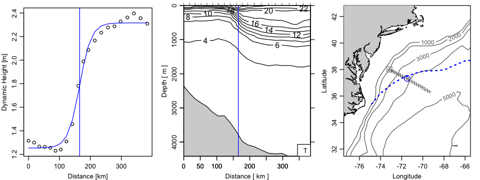
nnDefinitions of Gulf Stream location sometimes centre on thermal signature, but it might make sense to work with dynamic height instead. This is illustrated here, using a model for , with the distance along the transect. The idea is to select the halfway point in the function, where the slope is maximum and where therefore the inferred geostrophic velocity peaks.
nnMethods and results
nn | library(oce)n |
## Loading required package: methodsn## Loading required package: mapprojn## Loading required package: mapsn | data(section)n## Extract Gulf Stream (and reverse station order)nGS <- subset(section, 109<=stationId & stationId<=129)nGS <- sectionSort(GS, by="longitude")nGS <- sectionGrid(GS)n## Compute and plot normalized dynamic heightndh <- swDynamicHeight(GS)nh <- dh$heightnx <- dh$distancennpar(mfrow=c(1, 3), mar=c(3, 3, 1, 1), mgp=c(2, 0.7, 0))nplot(x, h, xlab="Distance [km]", ylab="Dynamic Height [m]")nn## tanh fitnm <- nls(h~a+b*(1+tanh((x-x0)/L)), start=list(a=0,b=1,x0=100,L=100))nhp <- predict(m)nlines(x, hp, col='blue')nx0 <- coef(m)[["x0"]]nnplot(GS, which="temperature")nabline(v=x0, col='blue')nn## Determine and plot lon and lat of midpointsnlon <- GS[["longitude", "byStation"]]nlat <- GS[["latitude", "byStation"]]ndistance <- geodDist(lon, lat, alongPath=TRUE)nlat0 <- approxfun(lat~distance)(x0)nlon0 <- approxfun(lon~distance)(x0)nplot(GS, which="map",n map.xlim=lon0+c(-6,6), map.ylim=lat0+c(-6, 6))npoints(lon0, lat0, pch=1, cex=2, col='blue')ndata(topoWorld)n## Show isobathsndepth <- -topoWorld[["z"]]ncontour(topoWorld[["longitude"]]-360, topoWorld[["latitude"]], depth,n level=1000*1:5, add=TRUE, col=gray(0.4))n## Show Drinkwater September climatological North Wall of Gulf Stream.ndata("gs", package="ocedata")nlines(gs$longitude, gs$latitude[,9], col='blue', lwd=2, lty='dotted')n |
Exercises
nnFrom the map, work out a scale factor for correcting geostrophic velocity from cross-section to along-stream, assuming the Drinkwater (1994) climatology to be relevant.
nnResources
nn- n
- n
Source code: 2014-06-22-gulf-stream-center.R
n n - n
K. F. Drinkwater, R. A Myers, R. G. Pettipas and T. L. Wright, 1994.n Climatic data for the northwest Atlantic: the position of the shelf/slopen front and the northern boundary of the Gulf Stream between 50W and 75W,n 1973-1992. Canadian Data Report of Fisheries and Ocean Sciences 125.n Department of Fisheries and Oceans, Canada.
n n
R-bloggers.com offers daily e-mail updates about R news and tutorials on topics such as: visualization (ggplot2, Boxplots, maps, animation), programming (RStudio, Sweave, LaTeX, SQL, Eclipse, git, hadoop, Web Scraping) statistics (regression, PCA, time series, trading) and more...